NumPy Notes
Page Contents
Preamble...
Numpy "...is the fundamental package for scientific computing with Python...". Good for fast maths... mostly due to vectorization (batch operation on datasets without needing loops) implemented in the compiled modules underneath the Python interface, which, where possible, will take advantage of hardware vectorization. A lot of the more complex underlying modules for things like linear algebra, matrix operations etc, are build using the help of oftware libraries, available under BSD style licences, such as BLAS and derivatives like LAPACK.
import numpy as np
References
- Python for Data Analysis, Wes McKinney, O'Reilly Media
- NumPy Beginner's Guide, Ivan Idris, Packt Publishing
- NumPy: creating and manipulating numerical data, scipy-lectures.org.
Arrays
Intro
The Python NumPy array object is ndarray. Create it using any iterable via, typically, the function np.array(). The most basic properties are dtype giving the underlying machine datatype, shapegiving the length of each dimension and ndim giving the number of dimensions...
>>> a = np.array([1,2,3,4])
>>> a
array([1, 2, 3, 4])
>>> a.dtype
dtype('int32')
>>> a.shape
(4,)
>>> a.ndim
1
>>>a.reshape((2,2))
array([[1,2],
       [3,4]])
Can also create Python NumPy arrays using functions such as zeros(), ones(), empty(), arange() and other array creation routines. Caution with empty(): it does not create a zeroed array... it could well be filled with junk!
Slices
Slicing ndarrays generally works like normal Python list slicing except for the rather important caveat that NumPy arrays slices are not, unlike Python lists, copies of the data. NumPy slices are like views into an array.
In the following code snippet a slice from array a is stored in b. If a were a list then b would contain an independent copy of the slice data. But in the example below we see that modifying b changes the data in a! Thus NumPy array slices are more like views into an array>>> a = np.array([1,2,3,4,5,6]) >>> b = a[2:4] #<< 'b' will be a VIEW into 'a' >>> b array([3, 4]) >>> b[:] = 111 >>> b array([111, 111]) >>> a array([1, 2, 111, 111, 5, 6]) #<< Modifying 'b' changes 'a'!!
To get a copy of the array slice, you would have to explicity tell NumPy to copy the data using the copy() function:
>>> a = np.array([1,2,3,4,5,6])
>>> b = a[2:4].copy() #<< Here we take a COPY
>>> b
array([3, 4])
>>> b[:] = 111
>>> b
array([111, 111])
>>> a
array([1, 2, 3, 4, 5, 6]) #<< Modifying 'b' does NOT change 'a' here
It is, however, worth noting, that this is not the case when assigning into an array slice. Take the following example...
>>> a = np.array([1,2,3,4,5,6])
>>> c = np.array([999,999])

>>> a[0:2] = c
>>> a
array([999, 999, 111, 111,   5,   6])

>>> c[:] = 0 #<< Modifying 'c' here will not change 'a'
>>> c
array([0, 0])

>>> a
array([999, 999, 111, 111,   5,   6])
Boolean Indexing
A few things to note:
- The boolean array must be of the same length as the axis it's indexing,
- The Python keywords "and" and "or" do not work with boolean arrays, use "&" and "|",
- Selecting data from an array by boolean indexing always creates a copy of the data, even if the returned array is unchanged.
For example, an array of student names and an array of their test scores. To select just the students with a score above, say, 70 percent, we would write the following Python code:
>>> import numpy as np
>>> a = np.array(['James', 'John', 'Mike', 'Mark', 'Oliver', 'Peter'])
>>> b = np.array([ 85,     56,     77,     88,     66,       88     ])

>>> b > 70
array([ True, False,  True,  True, False,  True], dtype=bool)

>>> a[b > 70]
array(['James', 'Mike', 'Mark', 'Peter'], dtype='|S6')
This concept extends to multi-dimensional arrays. Lets say each student has sat 4 exams and we want to to see exam scores for certain students. The Python code becomes...
>>> import numpy as np
>>> a = np.array(['James', 'John', 'Mike', 'Mark', 'Oliver', 'Peter'])
>>> b = np.array([[ 85,     56,     77,     88,     66,       54     ],
...               [ 66,     73,     65,     73,     28,       34     ],
...               [ 74,     56,     73,     74,     49,       56     ],
...               [ 35,     42,     54,     65,     87,       27     ]])

>>> mask = (a == 'James') | (a=='Oliver')
>>> mask
array([ True, False, False, False,  True, False], dtype=bool)

>>> b[:,mask]
array([[85, 66],
       [66, 28],
       [74, 49],
       [35, 87]])
It is also possible to mask rows...
>>> mask_rows = np.array([True, False, True, False])
>>> b[mask_rows]
array([[85, 56, 77, 88, 66, 54],
       [74, 56, 73, 74, 49, 56]])
In the above b[mask_rows] is equivalent to b[mask_rows, :]. Also note that the mask must also be a NumPy array, it cannot be, for example, a plain list... that won't work as you expect!
Index With Integers - Fancy Indexing
Use integers to specify which row/column to select and in what order
>>> a = np.array( [[0,1,2,3],[4,5,6,7],[8,9,10,11]] )
>>> a[[2,1], :]
array([[ 8,  9, 10, 11],
       [ 4,  5,  6,  7]])

>>> a[:, [2,1]]
array([[ 2,  1],
       [ 6,  5],
       [10,  9]])

>>> a[[2,1], [2,1]]
array([ 10, 5])
Condition Logic
The NumPy np.where() is the vectorized verions of the ternary "x if cond else y" operator.
np.putmask() replaces elements of an array based on conditions.
>>> x = np.arange(6).reshape(2, 3)
>>> np.putmask(x, x>2, x**2)
>>> x
array([[ 0,  1,  2],
       [ 9, 16, 25]])
Broadcasting
Broadcasting in Python works pretty much the same way as broadcasting in Yorick.
>>> a = np.array([1,2])
>>> b = np.array([a,a])
>>> a
array([1, 2])
>>> b
array([[1, 2],
       [1, 2]])
>>> a*b
array([[1, 4],
       [1, 4]])
>>> a+b
array([[2, 4],
       [2, 4]])
This is summarised very will in "Python For Data Analysis" as follows.
Two [Python NumPy] arrays are compatible for broadcasting if for each trailing dimension (that is, starting from the end), the axis lengths match or if either of the lengths is 1. Broadcasting is then performed over the missing and / or length 1 dimensions [1].
Stacking, Concatenating
Remember that a 3D array is indexed as [depth][row][col] because Python is row-major (i.e. fastest increasing index on the right).
>>> a = np.arange(8).reshape((2,2,2))
>>> a
array([[[0, 1],
        [2, 3]],

       [[4, 5],
        [6, 7]]])
>>> np.concatenate([a,a], axis=0)
array([[[0, 1],
        [2, 3]],

       [[4, 5],
        [6, 7]],

       [[0, 1],
        [2, 3]],

       [[4, 5],
        [6, 7]]])
>>> np.concatenate([a,a], axis=1)
array([[[0, 1],
        [2, 3],
        [0, 1],
        [2, 3]],

       [[4, 5],
        [6, 7],
        [4, 5],
        [6, 7]]])
>>> np.concatenate([a,a], axis=2)
array([[[0, 1, 0, 1],
        [2, 3, 2, 3]],

       [[4, 5, 4, 5],
        [6, 7, 6, 7]]])
Statistics (and how axis numbering works)
There are a few statistical measures that can be efficiently made across an array including the mean(), std(), var() and their not-a-number-ignoring equivalents nanmean(), nanstd(), nanvar(). These can be computed along any array "axis" or for the entire array...
I was a little surprised with how Python's NumPy labeled the axes... for 2D arrays here's how it works:
>>> a = np.arange(4).reshape(2,2)
>>> a
array([[0, 1],
       [2, 3]])
>>> a.mean()  # Compute mean of entire array
1.5
>>> a.mean(0) # Mean of each column
array([ 1.,  2.])
>>> a.mean(1) # Mean of each row
array([ 0.5,  2.5])
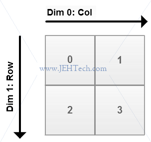
Because we index the 2D array as array[row][col] it makes sense to me that the column-axis number is 0 and the row-axis number is 1.
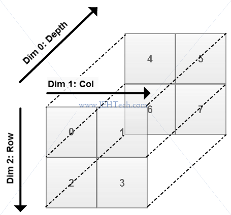
For 3D arrays it works like this...
>>> b = np.arange(8).reshape(2,2,2)
>>> b
array([[[0, 1],
        [2, 3]],
       [[4, 5],
        [6, 7]]])
>>> b.mean()  # Compute mean of entire array
3.5
>>> b.mean(0) # Mean of each depth
array([[ 2.,  3.],
       [ 4.,  5.]])
>>> b.mean(1) # Mean of each column
array([[ 1.,  2.],
       [ 5.,  6.]])
>>> b.mean(2) # Mean of each row
array([[ 0.5,  2.5],
       [ 4.5,  6.5]])
Note: The call b.mean(xxx) is the same as b.mean(axis=xxx).
The 3D array above is indexed as [depth][row][col] as Python is row-major (i.e. fastest increasing index on the right).
I had expected that the axes would numbered from zero, zero being the fastest increasing index (i.e., col). The next fastest increasing index (i.e, row) is numbered 1 and so on. Therefore, in this case axis 0 would be column, axis 1 would be row and axis 2 would be depth.
This is not the case as we can see!! The actual numbering makes sense if we think of a 1D array as being only rows, so the row-axis would be labeled 0. Adding a dimension causes all other axis to have their label incremented by 1 and the new axis to be labeled zero. This is how the axis numbering really works and this is what is shown in the image above.
Thus, a 1D array has only rows so the row-axis is labeled 0. A 2D array has a new dimension, columns. So increment the row column label so that it is now labeled 1. The new dimension (axis), column, is now labeled 0. A 3D array adds yet another dimension, depth. So increment the labels of the existing axes so that row now becomes 2, column 1, and the new axis 0.