Statistics Notes
Page Contents
References and Resources
"Introduction To Statistics", Thanos Margoupis, University of Bath, Peason Custom Publishing.
A technical book but quite dry (as most statistics books are!)
"An Adventure In Statistics, The Reality Enigma", Andy Field
A very entertaining book that explains statistics in a really intuitive way and uses examples that are actually slightly interesting!
The following are absolutely amazing, completely free, well taught resources that just put things in plain English and make concepts that much easier to understand! Definitely worth a look!
- The amazing Khan Achademy.
- The amazing CK12 Foundation.
The Basics of Discrete Probability Distributions
Some Terminology
Variables...
| Categorical Variable | Discrete variable which can be one of a set of such as the anwer to a YES/NO question: the variable can be either YES or NO. Or the answer to a quality question where the choices are good, ambivalent or bad, for example. |
| Consistent estimator | A consistent estimator is one that converges to the value being estimated. |
| Numerical Variable | Has a value from a set of numbers. That set can be continuous, like the set of real numbers, or discrete like the set of integers. |
| Random Variable | The numerical outcome of a random experiment. Discrete if it can take on more than a countable number of values. Continuous if it can take any value over an uncountable range. |
| I.D.D. | A sequence or other collection of random variables is independent and identically distributed (i.i.d.) if each random variable has the same probability distribution as the others and all are mutually independent. |
| Qualitative Data | Data where there is no measurable difference (in a quantitative sense) between two values (that makes sense). For example, the colour of a car. The car can be "nice" or "sporty", but we can't define the the difference in terms of a number like 4.83, for example. |
| Quantitative Data | Data is numerical and the difference between data is a well defined notion. For example, if car A goes 33 MPG and care B does, 40 MPG, then we can say the difference is 7MPG. |
| Ordinal Data | The value of the data has an order with respect to other possible values. |
Populations and samples...
It is always worth keeping in mind that probability is a measure describing the likelihood of an event from the population. It is not "in" the data set (or sample) obtained... a sample is user to infer a probability about a population parameter.
| Population | The complete set of items of interest. Size is very large, denoted N, possibly infinite. Population is the entire pool from which a statistical sample is draw. |
| Sample | An observed subset of the population. Size denoted n. |
| Random Sampling | Select n objects from population such that each object is equally likely to be chosen. Selecting 1 object does not influence the selection of the next. Selection is utterly by chance. |
| Parameter | Numeric measure describing a characteristic of the population. |
| Statistic | Numeric measure describing a characteristic of the sample. Statistics are used to infer population parameters. |
| Inference | The process of making conclusions about the propulation from noisy data that was drawn from it. Involves formulating conclusions using data and quantifying the uncertainty associated with those conclusions. |
Experiments...
| Random Experiment | Action(s) that can lead to |
| Basic Outcomes | A possible outcome from a random experiment. For example, flipping a coin has two basic outcomes: heads or tails. |
| Sample Space | The set of all possible basic outcomes (exhaustively) from a random experiment. Note that this implies that the total number of possible outcomes is, or can be, known. |
| Event | A subset of basic outcomes from a sample space. For example,
a dice roll has 6 basic outcomes, 1 through 6. The sample space
is therefore the set {1, 2, 3, 4, 5, 6}. The event
"roll a 2 or 3" is the set {2, 3}.
|
Distributions...
| Probability Mass Function (PMF) | When evaluation a n function gives the probability that a random variable takes the value n. Only associated with discrete random variables. Also note that the function descibes the population. |
| Probability Density Function (PDF) | Only associated with continuous random variables. The area between two limits corresponds to the probabilty that the random variable lies within those limits. A single point has a zero probability. Also note that the function descibes the population. |
| Cumulative Distribution Function (CDF) | Returns the probability that |
| Quantile | The |
Population And Sample Space
We have said that the population is the complete set of items of interest.
We have said that the sample space is the set of all possible outcomes (exhaustively) from a random experiment.
So I wondered this. Take a dice roll. The population is the complete set of possible items {1, 2, 3, 4, 5, 6}.
The sample space is the set of all possible outcomes, also {1, 2, 3, 4, 5, 6}. So here sample space and
population appear to be the same thing, so when are they not and what are the distinguishing factors between the two??
The WikiPedia page on sample spaces caused the penny to drop for me:
...For many experiments, there may be more than one plausible sample space available, depending on what result is of interest to the experimenter. For example, when drawing a card from a standard deck of fifty-two playing cards, one possibility for the sample space could be the various ranks (Ace through King), while another could be the suits (clubs, diamonds, hearts, or spades)...
Ah ha! So my population is the set of all cards {1_heart, 2_heart, ...,
ace_heart, 1_club, ...} but the sample space may be, if we are looking
for the suits, just {heart, club, diamond, spade}. So the population and
sample space are different here. In this case the sample space consists of cards
separated into groups of suites. I.e. the popultation has been split into 4
groups because there are 4 events of interest. These events cover the sample space.
In summary the population is the set of items I'm looking at. The sample space may or may not be the population... that depends on what question about the population is being asked and how the items in the population are grouped per event.
Classic Probability
In classic probability we assume all the basic outcomes are equally likely
and therefore the probability of an event, A, is the number of basic
outcomes associated with A divided by the total number of possible outcomes:
An example of the use of classical probability might be a simple bag of marbles. There are 3 blue marbles, 2 red, and 1 yellow.
If my experiment is to draw out 1 marble then the set of basic outcomes
is
{B1, B2, B3,
           R1, R2, Y1}
.
This is also the population!
Also, note that the sample space isn't
{B, R, Y} because we can differentiate between similar coloured
marbles and there is a certain quanity of each.
So, what is the probability of picking out a red. Well, here
What if my experiment is to draw 2 marbles from the sack? Now the set of all possible basic outcomes, if the order of draw was important would be a permutation. This means that if I draw, for example, R1 then B2, I would consider it to be a distinctly different outcomes to drawing B2 then R1. That means my population is:
| Selection 1 | Selection 2 | Selection 1 | Selection 2 |
| B1 | B2 | B2 | B1 |
| B1 | B3 | B2 | B3 |
| B1 | R1 | B2 | R1 |
| B1 | R2 | B2 | R2 |
| B1 | Y1 | B2 | Y1 |
| B3 | B1 | ||
| B3 | B2 | ||
| B3 | R1 | ||
| B3 | R2 | ||
| B3 | Y1 | ||
| R1 | R2 | R2 | R1 |
| R1 | B1 | R2 | B1 |
| R1 | B2 | R2 | B2 |
| R1 | B3 | R2 | B3 |
| R1 | Y1 | R2 | Y1 |
| Y1 | B1 | ||
| Y1 | B2 | ||
| Y1 | B3 | ||
| Y1 | R1 | ||
| Y1 | R2 |
Which is a real nightmare to compute by trying to figure out all the permutations by hand, and imagine, this is only a small set! Maths to the rescue...
And that is how many permutations we have in the above table (thankfully!).
So, if my question is what is the probability of drawing a red then a yellow
marble, my event space is the set
{R1Y1, R2Y1}.
Thus, if we say event A is "draw a red then a yellow marble",
What if we don't care about the order. What is the probability of drawing a red and a yellow? I.e. we consider RY and YR to be the same event...
Our event space therefore becomes:
{R1Y1, R2Y1
           Y1R1, Y1R2}
.
Thus, if we say event A is "draw a red and a yellow marble",
We are essentially now dealing with combinations.
Therefore in the above table, where we see things like...
| Selection 1 | Selection 2 |
| B1 | B2 |
| B2 | B1 |
...we can delete one of the rows. The set of all basic outcomes therefore becomes:
| Selection 1 | Selection 2 | Selection 1 | Selection 2 |
| B1 | B2 | ||
| B1 | B3 | B2 | B3 |
| B1 | R1 | B2 | R1 |
| B1 | R2 | B2 | R2 |
| B1 | Y1 | B2 | Y1 |
| B3 | R1 | ||
| B3 | R2 | ||
| B3 | Y1 | ||
| R1 | R2 | ||
| R1 | Y1 | R2 | Y1 |
Again a nightmare to figure out by hand, so maths to the resuce...
And, again, that is how many selections (not included the ones we've deleted using a strikethrough font) we have in the above table (thankfully!).
So, now we can't ask about drawing a red then a yellow
marble anymore as order doesn't matter. We can ask about drawing a red
and a yellow though.
My event space is now the set
{R1Y1, R2Y1
         Y1R1, Y1R2}
because I not longer care about order-of-draw...
Thus, if we say event A is "draw a red and a yellow marble",
We have noted that in classical probability that the various outcomes are equally likely. This means that from my bag of marbles am am equally likely to pick any marble. But what if this was not the case? What if the blue marbles are very heavy and sink to the bottom of the sack whilst the other marbles tend to rest on top of the blue marbles. We could hardly say that I am as likely to pick a blue as I am a red in this case. In this cas we cannot use classical probability to analyse the situation.
Relative Frequency Probability
Here the probability of an
event occurring is is the limit of the proportion of times an event occurs in
a large number of trials. Why the limit? Well, the limit would mean we tested
the entire population. Usually, however, we just pick a very large n
and infer the population statistic from that.
So, for example, if we flip a coin 1000 times there are 1000 total number of outcomes.
If we observed 490 heads and 510 tails we would have...
If the coin was entirely fair then we would expect an equal probability
of getting a head or a tail. Frequentist theory states that as the sample
size gets bigger, i.e., as we do more and more coin flips, if the coin
is fair the probabilities will tend towards 50%. So if we did 1,000,000
samples, for example, we might expect...
As n tends to infinity, we can say that n tends towards the population size, and then at this point you will arrive back at the formula for conditional probability you saw in the previous section
Event A OR Event B
What is independence? A and B are said to be independent if information on the value of A does not give any information on the value of B, and vice versa.
We can visualise this as follows, using a Venn diagram...
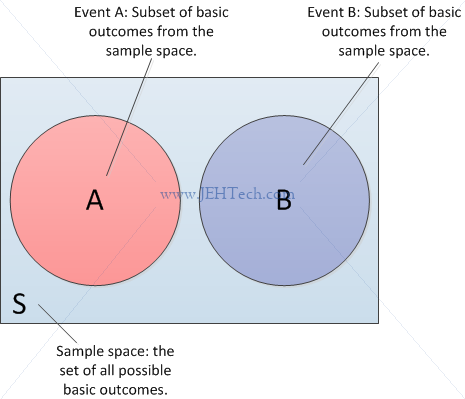
If two events are independent then we can see that none of the basic outcomes from either event can occur for the other.
Therefore, using either classical or relative-frequency probability we can see that
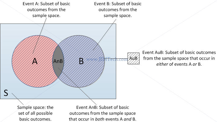
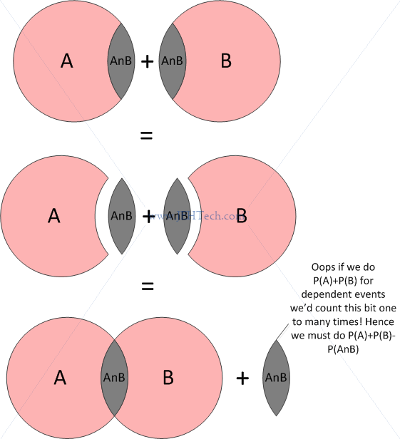
Now the two events are related. They are no longer independent because some of the basic outcomes from one event are also basic outcomes of the other. Thus we can see that if we sum the probabilities for the basic outcomes for each, we will count the shared basic outcomes twice!
If that's not clear, think of it this way...
Event A AND Event B
We just talked about independence, but how do we know if an event A, is
independent of another event, B? The answer is that two events are
indpendent if
Why is this? Let's think of this from the relative frequency point of
view. We know that
For every basic outcome in the set A, we can
pick an outcome from the set B, so the count of the combination of all possible
outcomes from both sets must be
So, what if the events are not independent? Then it is no longer true
that the count of combination of all possible outcomes is
Think if it this way. For A and B to both occur, at least one must have occurred, so now the only possible choices from the other event are in the overlapping region, not in the entire event space. Keep reading the next section on condition probability to find out more about why this is an indicator of independence.
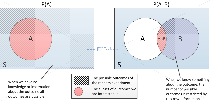
Event A GIVEN Event B
If I live with my partner it seems intuitively correct to say that the probability of myself getting a cold would be heightened if my partner caught a cold. Thus there is an intuitive difference between the probability I will catch a cold and the probability that I will catch a cold, given my partner has already caught one.
This is the idea behind conditioning: conditioning on what you know can change the probability of an outcome with no apriori knowledge of the data.
Lets look at a really simple example. I roll a dice... what is the probability
that I roll a 3. We assume a fair dice, so the answer is easy: 1/6.
The set all of basic outcomes was {1, 2, 3, 4, 5, 6} (the sample space) and only
one outcome was relevant for our event... so 1/6.
Now lets say I have rolled the dice and I have been informed that the
result was an odd number. With this knowledge, what is the probability that
I rolled a 3? The set of basic outcomes is now narrowed to {1, 3, 5}
and so the probability is now 1/3!
The probability of event A given that event B has occurred is denoted
This makes intuitive sense. If B has occurred then the number of outcomes
to "choose" from is represented by the circle for B in the
Venn diagram below. The number of of outcomes that can belong to event
A, given that we know event B has occurred, is the intersection.
Therefore, our sample space is really now all the outcomes for event B,
so
If A and B are independent then clearly, because
We can re-arrange the above to get another formula for
And now we can see why, if two events are independent that
A small bit on terminology...
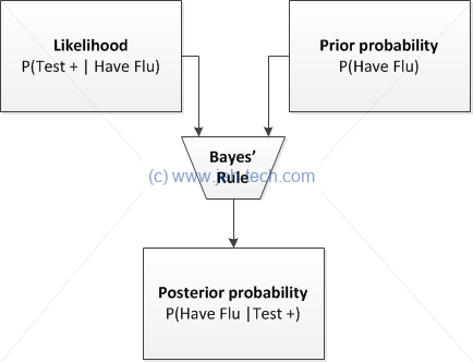
...A posterior probability is the probability of assigning observations
to groups given the data. A prior probability is the probability that
an observation will fall into a group before you collect the data. For
example, if you are classifying the buyers of a specific car, you might
already know that 60% of purchasers are male and 40% are female. If you
know or can estimate these probabilities, a discriminant analysis can
use these prior probabilities in calculating the posterior probabilities.
-- Minitab support
From the definitions so far we can also see that
Why is this important? Let's look at a little example. Say we have a
clinical test for Influenza. Imagine that we know that for a patient the
probability that they have or do not have Influenza.
Any clinical test is normally judged by it's sensitivity and specificity. Sensitivity is the probability that the test reports infection if the patient has Influenza (i.e true positives). Sepcificity is the probability that the test reports the all-clear if the patient does not have Influenza (i.e., true negatives).
Let's say the test has the following sensitivity and specificity respectively:
We can use the conditional probability formula to work this out...
Sensitivity v.s. Specificity
In clinical tests, the user often wants to know about the sensitivity of a test. I.e., if the patient does have the disease being tested for, what is the probability that that the test will call a positive results. Obviously, we would like this to be as close to 100% as possible!
The clinician would also like to know, if the patient did not have the disease, what is the probability that the test calls a negative. Again, we would like this to be as close to 100% as possible!
To summarise: sensitivity is the probability of a true positive, and specificity is the probability of a true negative.
Sensitivity:
Specificity:
Compliments
Bayes' Theorem
Recall the multiplication rule:
Because we know that
Remember that we called
Alternative Statement
This can sometimes be usefull re-stated as follows. If all events
Discrete Probability Distributions
General Definitions
The Probability Mass Function (PMF) is another name for the Probability
Distribution Function (PDF),
The Cumulative Mass Function (CMF) or Cumulative Probability Function (CPF),
Expected Value and Variance
Expected value defined as:
The calculation of measurements like
Variance,
Standard Deviation,
The calculation of measurements like
Why does
For example, lets say that we have weighted dice so that the probabilities are as follows:
| Value | Probability |
| 1 | 0.05 |
| 2 | 0.1 |
| 3 | 0.1 |
| 4 | 0.1 |
| 5 | 0.1 |
| 6 | 0.55 |
The population mean,
Linear Functions Of X
The expected value and variance of a linear function of
| g(x) | Probability |
| 7 | 0.05 |
| 9 | 0.1 |
| 11 | 0.1 |
| 13 | 0.1 |
| 15 | 0.1 |
| 17 | 0.55 |
The expected value of
We can derive the first equation as follows, using our first definition
of the expected value of a random variable.
Binomial Distribution
Bernoulli Model
Experiment with two mutually exclusive and exhaustive outcomes. One has
the probability
Binomial Distribution
Bernoulli experiment repeated
We know from previous discussions that if two events are independent
then
Let's take a simple example. I have a bag with 5 balls in it: 3 blue, 2 red. What is the probability of drawing 1 blue ball and 1 red ball if I select using replacement (to make the selections independent). Replacement means that what ever ball I pick first, I record the result and then put it back in the bag before making my next pick. In this way, the probability of selecting a particular colour does NOT change per pick.
Note that there are only 2 colours of ball in our bag... this is because we are talking about an experiement where there are only two outcomes, labeled "success" and "failure". We could view selecting a blue as "success" and a red as "failure", or vice versa.
So... selecting a blue and a red ball. Sounds like
Here I am using an alphabetical subscript to indicate the specific ball. I.e.
| ... | |||||
There are two clear groups of outcomes that will satisfy the question.
We see that in one group we drew a red ball first and in the other we
drew a blue ball first. So, there are
This confusion can be resolved by careful attention to definitions and notation.
Where you write
The events you are interested are
You want to know
Note, that in Jorki's example
So, having understood this, we can see that to get the total probability
of
The formula for the binomial distribution is...
This, incidentally is the same as asking for
Let's do this to exhaustion... let's imagine another bag. It doesn't
matter how many blue and red balls are in there, just so long as I can
select 3 blue balls and 1 red.
We can draw a little outcome tree as follows:
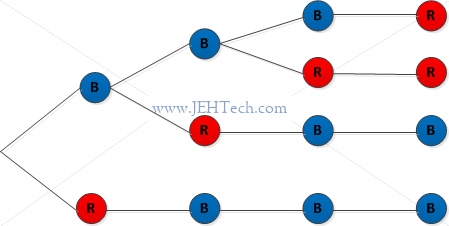
Clearly there are 4 ways to arrive at the selection of 3 blues and 1 red,
once we have made that particular selection. Remember we're not asking
for a blue/red on a specific turn... we just care about the final
outcome, irrespective of the order in which the balls were picked.
And we can see...
Why don't we use permutations? The answer is that we don't care if we got
Having gone through this we can then use the formulas for expected value,
or mean, and variance. To make the notation similar to previous examples
where we used
Recalling that
The population mean and variance are summarised as follows.
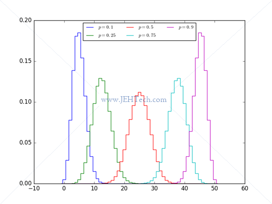
Often when talking about a binomial distribution you will see something like
We can plot some example distributions... lets do this using Python.
import matplotlib.pyplot as pl
import numpy as np
from matplotlib.font_manager import FontProperties
from scipy.stats import binom

fontP = FontProperties()
fontP.set_size('small')

n=50
pLst=[0.1, 0.25, 0.5, 0.75, 0.9]
x = np.arange(-1, n+2)
fig, ax = pl.subplots()

for p in pLst:
   dist = binom(n, p)
   ax.plot(x, dist.pmf(x),linestyle='steps-mid')

ax.legend(['$p={}$'.format(p) for p in pLst],
          ncol = 3,
          prop=fontP,
          bbox_to_anchor=[0.5, 1.0],
          loc='upper center')
fig.show()
fig.savefig('binomial_distrib.png', format='png')
Poisson Distribution
Didn't like the starting explanation in [1] so had a look on Wikipedia and found a link to the UMass Amherst Uni's stats page on the Poisson distribution which I though was really well written. That is the main reference here.
Poisson distribution gives the probability of an event occuring some number of times in a specific interval. This could be time, distance, whatever. What matters is that the interval is specific and fixed.
The example used on the UMass Amherst is letters received in a day. The interval here is one day. The poisson distribution will then tell you the probability of getting a certain number of letters in one day, the interval. Other examples could include the number of planes landing at an airport in a day or the number of linux server crashes in a year etc...
The interval is one component. The other is an already observed average
rate per interval, or expected number of successes in an interval,
So, poisson has an interval and an observed average count for that interval. The following assumptions are made:
- The #occurrences can be counted as an integer
- The average #occurrences is known
- The probability of the occurence of an event is constant for all subintervals. E.g., if we divided the day into minutes, the probability of receiving a letter in any minute of the day is the same as for any other minute.
- There can be no more than one occurrence in the subinterval
- Occurrences are independent
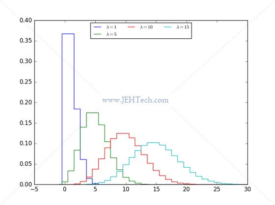
The distribution is defined as follows, where
Eek... didn't like the look of trying to derive the mean and variance.
The population mean and variance are as follows.
We can plot some example distributions... lets do this using Python.
import matplotlib.pyplot as pl
import numpy as np
from matplotlib.font_manager import FontProperties
from scipy.stats import poisson

fontP = FontProperties()
fontP.set_size('small')

expectedNumberOfSuccessesLst = [1, 5, 10, 15]
x = np.arange(-1, 31)
fig, ax = pl.subplots()

for numSuccesses in expectedNumberOfSuccessesLst:
   ax.plot(x, poisson.pmf(x, numSuccesses),linestyle='steps-mid')

ax.legend(['$\lambda={}$'.format(n) for n in expectedNumberOfSuccessesLst],
          ncol = 3,
          prop=fontP,
          bbox_to_anchor=[0.5, 1.0],
          loc='upper center')
fig.show()
pl.show()
fig.savefig('poisson_distrib.png', format='png')
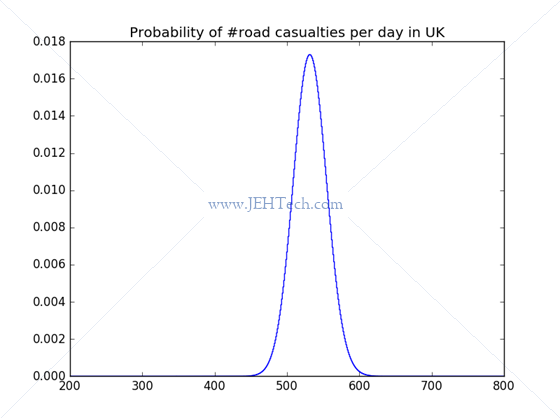
Lets take a little example. Looking at the UK government report on road casualties in 2014, there were a reported 194,477 casualties in 2014. This gives us an average of 532.8137 (4dp) casualties per day! So, we could ask some questions...
What is the probability that no accidents occur on any given
day? Recalling that...
Of course, we could critisize this analysis as not taking into account seaons, or weather conditions etc etc. In winter, for example, when the roads are icy one might expect the probability of an accident to be greater, but for the purposes of a little example, I've kept it simple.
We might also ask, what is the probability that the number of casualties
is less than, say, 300?
from scipy.stats import poisson
print poisson.cdf(299, 194477.0/365)
This outputs
import matplotlib.pyplot as pl
import numpy as np
from scipy.stats import poisson

x = np.arange(200, 800)
fig, ax = pl.subplots()
ax.plot(x, poisson.pmf(x, 194477/365), linestyle='steps-mid')
ax.set_title('Probability of #road casualties per day in UK')
fig.show()
fig.savefig('poisson_road_fatilities_distrib.png', format='png')
Joint Distributions
When one thing is likely to vary in dependence on another thing. For example, the likely longevity of my milk will correspond to some extent to the temperature of my fridge: there is a relationship between these two variables so it is important that any model produced includes the effect of this relationship. We need to define our probabilities that random variables simultaneously take some values.
Enter the joint probability function. It expresses the probability that each random variable takes on a value as a function of those variables.
A two variable joint probability distribution is defined as:
The marginal probabilities are the probabilities that one random
variable takes on a value regardless of what the other(s) are doing. In
our two variable distribution we have:
Joint probability functions have these properties:
- The sum of the join probabilities is 1.
The conditional probability function looks like this...
The random variables are independent if their joint
probability function is the product of their marginal probability
functions:
The conditional mean and variance are:
Covariance and Correllation
Measure of joint variablility: the nature and strength of a relationship between two variables.
Covariance between two random variables
Correlation is just a "normalisation" of the
covariance such that the measure is limited to being in the range [-1, 1].
This YouTube video explains the difference really well:
Continuous Distributions
Cumulative Distribution Function (CDF)
CDF gives probability that continuous random variable
To get the probability that
Probability Density Function (PDF)
Call our PDF
Uniform Distribution
The uniform distribution is one where the probability that
Normal Distribution
This distribution is defined by a gaussian bell-shaped curve.
The probability distribution function for a normally distributed random vairable,
- About 68% of the data will fall within one standard deviation,
- About 95% of the data will fall within two standard deviations,
- Over 99% of the data will fall within three standard deviations,
- Mean is
- Variance is
The normal distribution is defined with the following notation:
The standard normal distribution is a normal distribution where
the the mean is 0 and the variance is 1:
To solve
We can also get the probability of a Z score and vice versa in Python
by using scipy.stats.norm.cdf() and scipy.stats.norm.ppf()
respectively as documented here.
Percentiles
Wikipedia defines a percentile as a measure giving the value below which a given percentage of obersvations fall. If an observation is AT the xth percentile then it has the value, V, at which x% of the scores can be found. If it is IN this percentile then its value is in the range 0 to V.
Percentiles aren't really specific to normal distributions but you often get asked questions like "what is the 95th percentile of this distribution?"
In the standard normal distribution...
- 90th percentile is at z=1.28. (This is because
- 95th percentile is at z=1.645. (This is because
- And so on...
Sampling Distributions
A Little Intro...
So far we have been talking about population statistics. The
values
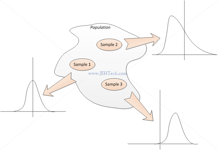
So, what is normally done is to take a sample from the population and then use the sample statistics to make inferences about the population statistics. The image below shows three samples that have been taken from a population. Each sample set can, and will most probably, have a different shape, mean, and variance!
We can demonstrate this concept using a quick little Python program to take 4 samples from the normal distribution where each sample has 10 members:
import numpy as np
import matplotlib.pyplot as pl

numSampleSets = 4
numSamplesPerSet = 10

# Limit individual plots, otherwise the first plot takes forever and is rubbish
doShowIndividualSamples = (numSampleSets <= 8) and (numSamplesPerSet <= 50)

# Create a numSampleSets (rows) x numSamplesPerSet (cols) array where we use
# each row as a sample.
randomSamples = np.random.randn(numSampleSets, numSamplesPerSet)

# Take the mean of the rows, i.e. the mean of each sample set
means = randomSamples.mean(axis=1)

if doShowIndividualSamples:
   fig, axs = pl.subplots(nrows=int(numSampleSets/2.0+0.5), ncols=2)
   xticks = np.arange(numSamplesPerSet, dtype='float64')
   for idx in range(numSampleSets):
         ax_col = idx % 2
         ax_row = int(idx/2.0)
         thisAx = axs[ax_row][ax_col]
         thisAx.bar(xticks, randomSamples[idx][:], width=1)
         thisAx.set_xticks(xticks + 0.5)
         thisAx.set_xticklabels(xticks, fontsize=8)
         thisAx.axhline(y=means[idx], color="red", linewidth=2)
         thisAx.set_title("Sample set #{}".format(idx))
         thisAx.grid()

xticks = np.arange(numSampleSets, dtype='float64')
fig2, ax2 = pl.subplots(nrows=2)
ax2[0].bar(xticks, means)
ax2[0].grid()
ax2[0].set_title("Distribution of {} sample means (n={})".format(numSampleSets, numSamplesPerSet))
ax2[0].set_ylabel("Mean value")
ax2[0].set_xlabel("Sample set #")

ax2[1].hist(means, 50)
ax2[1].grid()
ax2[1].set_title("Histogram of {} sample means (n={})".format(numSampleSets, numSamplesPerSet))
ax2[1].set_ylabel("# sample mean's")
ax2[1].set_xlabel("Sample mean bin")

pl.tight_layout()
pl.show()
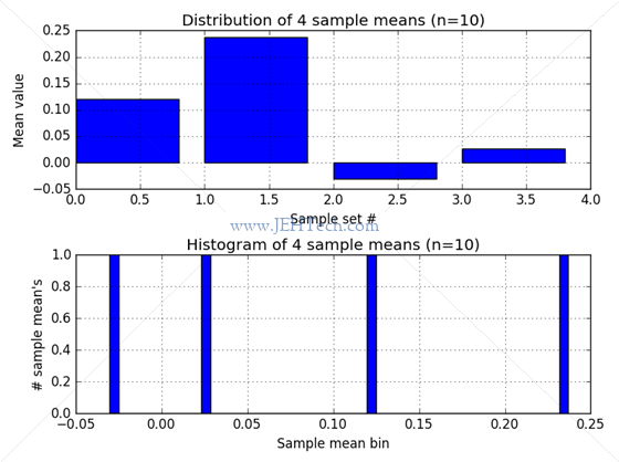
The script above produces the following graphs. The x-axis is just the sequence number of the sample member and the y-axis the value of the sample member. The horizontal line is the sample mean.
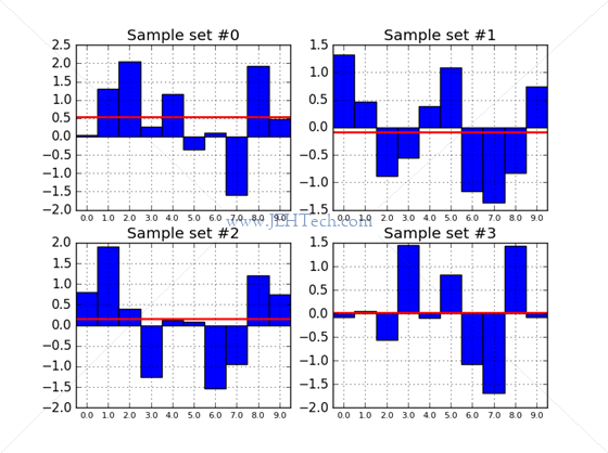
We can see from this little example that the samples in each of the 4 instances are different and that the mean is different for each sample. Keep in mind that the graph shown when you run the above script will be different as it is a random sample :)
So we can see that although the population mean is fixed the sample mean can vary from sample to sample. Therefore, the mean of a sample is itself a random variable and as a random variable it will have it's own distribution (same applies for variance).
But, we want to use the sample statistics to infer the population statistics. How can we do this if the sample mean (and variance) can vary from sample to sample? There are a few key statistical theories that will help us out...
Independent and Identically Distributed (I.I.D.) Random Variables
Wikipedia says that ...a sequence or other collection of random variables is independent and identically distributed (I.I.D.) if each random variable has the same probability distribution as the others and all are mutually independent...
It is often the case that if the population is large enough and a sample from the population only represents a "small" fraction of the population that a set of simple random samples without replacement still qualifies I.I.D. selections. If you sample from a population and the sample size represents a significant fraction of the population then you cannot assume this to be true.
We're going to need to know this a little later on when we talk about conistentent estimators and the law of large numbers...
The Law of Large Numbers
The law of large numbers states that the average of a very large number (note we haven't quite defined what "very large" is) of items will tend towards the average of the popultion from which the items are drawn. I.e., the sample mean (or any other parameter) tends towards the population mean (or parameter, in general) as the number of items in the sample tends to infinity.
This is shown empirically in the example below:
import numpy as np
import matplotlib.pyplot as pl

maxSampleSizes = [100, 1000, 100000]
fig, axs = pl.subplots(nrows = 3)
for idx, ssize in enumerate(maxSampleSizes):
   sample_sizes = np.arange(1,ssize+1)
   sample_means = np.random.randn(ssize).cumsum() / sample_sizes
   axs[idx].plot(sample_sizes, sample_means)
   axs[idx].set_xlabel("Sample size, max is {}".format(ssize));
   axs[idx].set_ylabel("Average")
   axs[idx].axhline(y=0, color="red")

fig.show(); pl.show()
Explain the code a little... np.random.randn(ssize) generates a
numpy array with ssize elements. Each element is a "draw" from
the standard normal distribution. The function cumsum() then
produces an array of ssize elements where the second element is
the sum of the first 2 elements, the third element is the sum of the first 3 elements
and so on. Thus we have an array where the ith element is the
sum of i samples. Dividing this by the array sample_sizes
gives us an array of means where the ith element is the mean of
a sample with i items.
Running the code produced the figure below...
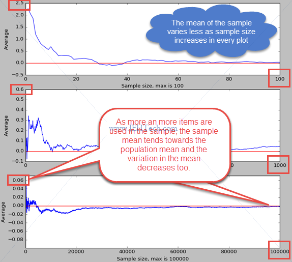
To summarise, the law of large numbers states that the sample mean of I.I.D. samples is consistent with the population mean. The same is true for sample variance. I.e., as the number of items in the sample increases indefinitely, the sample mean will become a better and better estimate of the population mean.
Sampling Distribution Of The Sample Mean
We've established that between samples, the mean and variance of the samples, well... varies! This implies that we can make a distribution of sample means.
The "sampling distribution of the sample mean" (a bit of a mouthful!) is the probability distribution of the sample means obtained from all possible samples of the same number of observations.
That's a bit of a mounthful! What it
means is that if we took, from the population, the exhaustive set of all
distinct samples of size
For example if I am a factory owner and I produce machines that accurately measure distance, I could have a population of millions. I clearly do not want to test each and every device coming off my production line, especially if the time that testing requires is anything approaching the time taken to produce the item: I'd be halving (or more) my production throughput!
So what do I do? I can take a sample of say 50 devices each day. I can test these to see if they accurately measure distance, and if they do I can assume the production process is still running correctly.
But as we have seem if I test 50 devices each day for 10 days, each of my 10 sample sets will have a different mean accuracy. On the first day, the mean accuracy of 50 devices might be 95%, on the second day, the mean of the next 50 devices might be 96.53% and so on.
The sample mean has a distribution. As we can take many samples from a population we have sampled the sample mean, so to speak, hence the rather verbose title "sampling distribution of the sample mean".
Now, I can ask, on any given day, "what is the probability that the mean accuracy of my 50 devices is, say 95%?". This is the sampling distribution of the sample mean: the probability distribution of the sample means (mean accuracy of a sample of devices) obtained from all possible samples (theoretical: we can't actually measure all possible samples!) of the same number of observations (50 in this case).
The law of large numbers gives us a little clue as to how variable the sample means will be... we know that if the sample size is large then the sample mean tends towards the population mean as has a much narrower variance about the population mean. So, 50 samples is better than 10. But 10,000 samples would be even better. The question is how many samples do we need. Will try to answer that (much) later on...
Sample Mean And It's Expected Value (The Mean Of Sample Means)
Continuing with the example of distance measurement devices. We could
say each device in our sample set is represented by random variables
Now we can calculate the expected value of the sample mean,
Imagine that
we take
A single sample mean can therefore be larger or smaller than the population mean, but on average, there isn't any reason to expect that it is either. As the sample size increases we also know that the likelihood of the sample mean being higher or lower than the population mean decreases (law of large numbers).
The Variance Of The Sample Mean w.r.t. Sample Size And Standard Error
Sample
variance can be written as
How did we get the above results? Well, it all is a bit brain melting, but
here goes. The variance of the mean of sample means is written as
The sample standard deviation is often refered to as the standard error.
The Shape Of The Samplign Distribution Of Sample Means
When samples are selected from a population that has a normal distribution we will see (anecdotally) that the sampling distribution of sample means is also normally distributed.
A histogram of the sample means gives a better picture of the distribution of sample means from the 4 sample sets. Diagrams have been drawn using the previous python example.
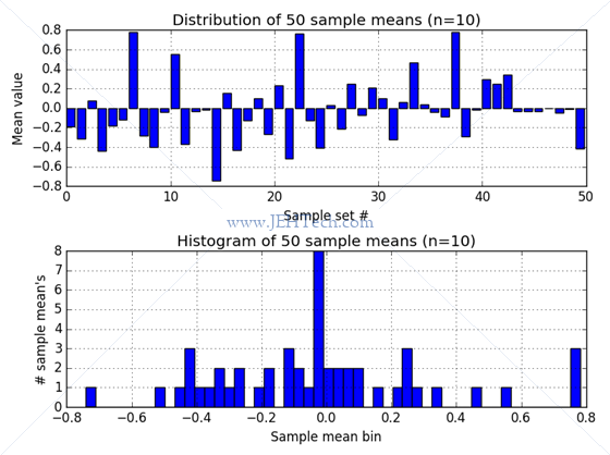
Now observe what happens when we increase the number of sample sets taken to 50. The distribution of sample means is still pretty distributed without much definition of the shape of the distribution...
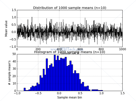
Now observe what happens when we increase the number of sample sets taken to 1000. The distribution of sample means begins to take shape...
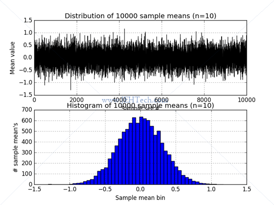
Now observe what happens when we increase the number of sample sets taken to 1000. The distribution of sample means now really looks very much like a gaussian distribution... interesting!
Clearly when we sample from the population the sample can be, to varying degrees, either a good or bad representation of the population. To help ensure that that sample represents the population (i.e., no "section" of the population is over or under represented) a simple random sample is usually taken.
Also of great interest in the above is that as the number of samples taken increases the distribution of sample means appears to become more and more gaussian in shape!. What is always true, and even more important is that the sampling distribution becomes concentrated closer to the population mean as the sample size increases, as we have seen in the maths earlier. The example above also doesn't proove it... its just anecdotal evidence. We could also notice that as #samples increases the variance of the sample mean decreases, again as we saw in the maths earlier.
Remember: take care to differentiate between the sample mean,
We must also remember to differentiate between the sample variance,
Also remember that the samples were drawn from a population that is normally distributed. So the sampling distribution was also normally distributed, as we have anacdotally seen. The central limit theory (CLT) will show us that is doesn't matter what the population distriution is. Enough samples and the sampling distribution of the sample mean will always tend towards normal distribution.
Because the sampling distribution of sample means is normally distributed,
it means that we can also form a standard normal distribution for the
sample means, which we do as follows:
Central Limit
We saw that the mean of the sampling distribution of sample means is
The central limit theorem removes the restriction that the population we
draw from need be normally distributed in order for the sampling distribution
of the sample mean to be normally distributed. The central limit theoem
states that the mean of a random sample drawn from a population with
any distribution will be approx. normally distributed as the
number of samples,
We could test this for, say, samples drawn from the binomial distribution. We have to modify our python code a little though (and also slim line some of the bits out)...
import numpy as np
import matplotlib.pyplot as pl

numSampleSets = 4000
numSamplesPerSet = 10
p = 0.5

# Make an array of numSampleSets means of samples of size numSamplesPerSet
# drawn from the binomial distirbution with prob of success `p`
means = np.random.binomial(numSamplesPerSet, p, numSampleSets)
means = means.astype("float64") / numSamplesPerSet

xticks = np.arange(numSampleSets, dtype='float64')
fig2, ax2 = pl.subplots()
ax2.hist(means, 50)
ax2.grid()
ax2.set_title("Histogram of {} sample means (n={})\nSamples draw from binomian p={}".format(numSampleSets, numSamplesPerSet, p))
ax2.set_ylabel("# sample mean's")
ax2.set_xlabel("Sample mean bin")

pl.tight_layout()
pl.show()
When we set the number of sample sets taken to be small, at 10, we get this:
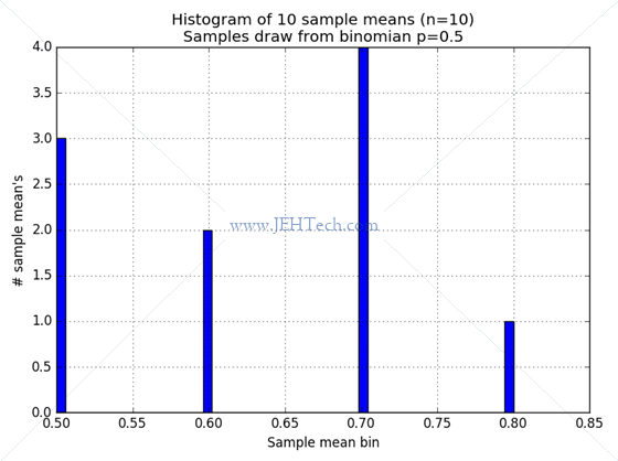
When we set the number of sample sets taken to be very large, at 4000, we get this:
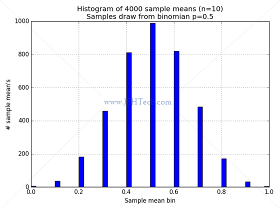
Hmmm... anacdotally satisfying at least.
Confidence Intervals
The following is mostly based on this Khan Achademy tutorial with some additions from my reference textbook.
A confidence interval is a range of values which we are X% certain contain an unknown population parameter (e.g. the population mean), based on information we obtain from a sample. In other words, we can infer from our sample something about an unknown population parameter.
Let's go back to our distance measurement devices. I have a test fixture that is exactly 100cm wide. Therefore a device should, when placed in this fixture, report/measure a distance of 100cm +/- some tolerance.
Remember that I don't want to test all of the sensors I've produced because this will kill the manufacturing time and significantly raise the cost per unit. So I've decide to test, let's say, 50 sensors.
As I test each device in my sample of 50 I will get back a set of test readings, one for each device. 100.1cm, 99cm, 99.24cm, ... etc. From the sample I can calculate sample mean and sample variance. But this is about all I know: I do not know my population mean or population variance!
But I have learn't something about the sampling distribution of sample means.
To recap, we have seen that:
So, I also know that my specific sample mean must lie somewhere in the sampling distribution of sample means...
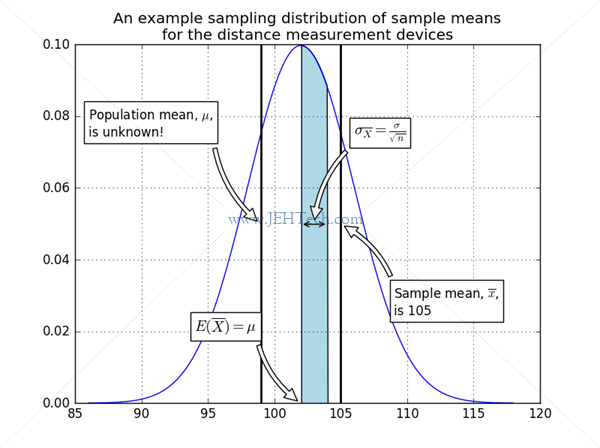
Continuing with the example then... let's say I have taken my sample
of 50 devices. I have a sample mean of
<Click me to toggle code view for graph creation>
import matplotlib.pyplot as pl
import numpy as np
import scipy.stats

sample_mean = 105
population_mean = 99
expected_sample_mean = 102
var_of_expected_sample_mean = 4
std_of_expected_sample_mean = np.sqrt(var_of_expected_sample_mean)

x = np.linspace( expected_sample_mean - 4 * var_of_expected_sample_mean
               , expected_sample_mean + 4 * var_of_expected_sample_mean
               , 500)
y = scipy.stats.norm.pdf( x
                        , loc   = expected_sample_mean
                        , scale = var_of_expected_sample_mean)

max_y = scipy.stats.norm.pdf( expected_sample_mean
                            , loc   = expected_sample_mean
                            , scale = var_of_expected_sample_mean)

fig, ax = pl.subplots()
ax.plot(x,y)
fill_mask = (x >= expected_sample_mean) & (x <= expected_sample_mean + std_of_expected_sample_mean)
ax.fill_between(x, 0, y
               , where       = fill_mask
               , interpolate = True
               , facecolor   = 'lightblue')

ax.annotate(r'$E(\overline{X}) = \mu$',
            xy=(expected_sample_mean, 0),
            xytext=(expected_sample_mean-2*var_of_expected_sample_mean, 0.02),
            bbox=dict(fc="w"),
            fontsize='large',
            arrowprops=dict(facecolor='black', shrink=0.05, connectionstyle="arc3,rad=0.2", fc="w"))


ax.annotate(''
      , xy=(expected_sample_mean, max_y/2)
      , xytext = (expected_sample_mean + std_of_expected_sample_mean, max_y/2)
      , arrowprops=dict(arrowstyle="<->"
                       , connectionstyle="arc3"
                       )
      )

ax.annotate(r'$\sigma_{\overline{X}} = \frac{\sigma}{\sqrt{n}}$',
            xy=(expected_sample_mean + std_of_expected_sample_mean/2, max_y/2),
            xytext=(expected_sample_mean + 2*std_of_expected_sample_mean, 3*max_y/4),
            fontsize='large',
            bbox=dict(fc="w"),
            arrowprops=dict(facecolor='black', shrink=0.05, connectionstyle="arc3,rad=0.2", fc="w"))


ax.axvline(x=population_mean, color='black', lw=2)
ax.annotate('Population mean, $\\mu$,\nis unknown!',
            xy=(population_mean, max_y/2),
            xytext=(x[0], 3*max_y/4),
            bbox=dict(fc="w"),
            arrowprops=dict(facecolor='black', shrink=0.05, connectionstyle="arc3,rad=0.2", fc="w"))

ax.axvline(x=sample_mean, color='black', lw=2)
ax.annotate('Sample mean, $\\overline{{x}}$,\nis {}'.format(sample_mean),
            xy=(sample_mean, max_y/2),
            xytext=(sample_mean + 2*std_of_expected_sample_mean, max_y/4),
            bbox=dict(fc="w"),
            arrowprops=dict(facecolor='black', shrink=0.05, connectionstyle="arc3,rad=0.2", fc="w"))

ax.set_title("An example sampling distribution of sample means\nfor the distance measurement devices")
ax.grid()
pl.show()
The graph above also shows the population mean. This also lies somewhere in this distribution of sample means, but we don't know where. This is the parameter that we want to infer! The single sample's mean and variance are all we have at the moment so somehow we need to move from these statistics to an assertion about the population mean.
Now I'm going to stop talking about
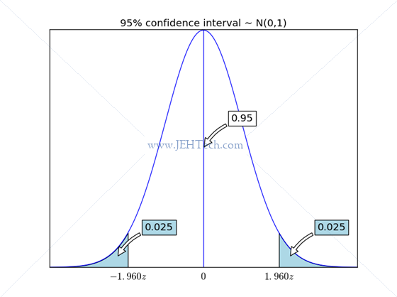
We know
Hang on! We know from the CLT that the sampling distribution should be normal. So we can figure this out using the normal distribution. Further more we know that we can normalise the distribution to arrive at the standard normal distribution. Therefore, what we are looking for in the standard normal is the following:
<Click me to toggle code view for graph creation>
import matplotlib.pyplot as pl
import numpy as np
import scipy.stats


z = np.linspace(-4, 4, 500)
y = scipy.stats.norm.pdf(z)
x_95p = scipy.stats.norm.ppf(0.975) #.025 in each tail gives 0.05 for 95% conf
x95_mid = scipy.stats.norm.ppf(0.9875)

fig, ax = pl.subplots()
ax.plot(z,y)
ax.fill_between(z, 0, y
               , where       = z < -x_95p
               , interpolate = True
               , facecolor   = 'lightblue')
ax.text(-x_95p, -0.02, "$-{0:.3f}z$".format(x_95p), ha="center", fontsize='large')

ax.fill_between(z, 0, y
               , where       = z > x_95p
               , interpolate = True
               , facecolor   = 'lightblue')
ax.text(x_95p, -0.02, "${0:.3f}z$".format(x_95p), ha="center", fontsize='large')

ax.plot( [0, 0], [0, max(y)], color='b')
ax.text(0, -0.02, "$0$", ha="center", fontsize='large')

ax.annotate( "0.025"
           , xy=(x95_mid, scipy.stats.norm.pdf(x95_mid)/2)
           , xytext=(40, 40)
           , textcoords='offset points'
           , bbox=dict(fc="lightblue")
           , fontsize='large'
           , arrowprops=dict(facecolor='black', shrink=0.05, connectionstyle="arc3,rad=0.2", fc="w"))

ax.annotate( "0.025"
           , xy=(-x95_mid, scipy.stats.norm.pdf(-x95_mid)/2)
           , xytext=(40, 40)
           , textcoords='offset points'
           , bbox=dict(fc="lightblue")
           , fontsize='large'
           , arrowprops=dict(facecolor='black', shrink=0.05, connectionstyle="arc3,rad=0.2", fc="w"))

ax.annotate( "0.95"
           , xy=(0, max(y)/2.0)
           , xytext=(40, 40)
           , textcoords='offset points'
           , bbox=dict(fc="w")
           , fontsize='large'
           , arrowprops=dict(facecolor='black', shrink=0.05, connectionstyle="arc3,rad=0.2", fc="w"))

ax.set_xticks([])
ax.set_yticks([])
ax.set_title("95% confidence interval ~ N(0,1)")
pl.show()
And we previously saw how to do this:
Quite a few assumptions and estimates have been made here. I assumed that I could estimate the population standard deviation with my sample's standard deviation. This could be okay for large sample sizes from an even larger population, but when this is not the case, this assumption breaks down. Something called the "Student-t" distribution will cope with this and we'll come to that later.
Kalman Filter
ttp://www.bzarg.com/p/how-a-kalman-filter-works-in-pictures/