• R Language Definition.
• The Art Of R Programming.
• Producing Simple Graphs with R, by Frank McCown

Getting Help

To get help on a function you can use the following...

?func-name               ## Display help for function with this exact name
help.search("func name") ## Search all help for function like this
args("func name")        ## gets args for this exact function

Typing a function name without the ending curley brackets displays the code for the function.

Working Directory

Functions will generally read or write to your working directory (unless you use absolute paths)

Use getwd() to display your current working directory and setwd("...") to set your current working directory. dir("...") will list a directory.

Source R code from console

Use source("..filename..").

If-then-else

If-the-else as standard...

if(...) {
} else if {
} else {
}

You can also assign from an if into a variable...

> x <- if(FALSE) { cos(22) } else { sin(22) }
> x
[1] -0.008851309
> x <- if(TRUE) { cos(22) } else { sin(22) }
> x
[1] -0.9999608

For loops

For each value in a range...

for(i in 1:10) { ... }

To generate an index for each member of a vector...

for(i in seq_along(x)) {
   ...x[i]...
}

For each item in a list...

for(item in x) { ... }

While loops

count <- 0
while(count < 10) {
   count <- count + 1
}

Infinite loops

repeat {
   // infinite loop
}

Skip loop iteration or exit loop

The standard break statement, and to continue use next

The basics...

In R, functions are first class objects which means that they can be passed as args to other functions. Functions can also be nested.

First class means that functions can be operated on like any other R object. I.e., ...this means the language supports passing functions as arguments to other functions, returning them as the values from other functions, and assigning them to variables or storing them in data structures... (Wikipedia article "First class functions").

Function arguments evaluated lazily, which means that they are only evaluated as they are needed/used.

Functions are declared as follows and return whatever the last statement evaluates to...

five <- function() {
+     1 + 4
+ }
> five()
[1] 5

Like many scripting langauges, function parameters can be declared too, and with default parameters

> threshold <- function(x, n=5) {
+    x[x > n] = n
+    x
+ }
> threshold(1:10, 2)
 [1] 1 2 2 2 2 2 2 2 2 2

Also like many other languages, functions can accept a variable number of arguments, using the C-like syntax of three consequitive dots, or "ellipsis". For more information read this r-bloggers article.

The '...' argument indicates variable number of arguments. You can pass the list using '...' to other functions as well. Note that arguments after '...' must be named explicitly and cannot be partially matched.

> test <- function(...) {
+    arguments <- list(...)
+    arguments
+ }

> test(1,2, a=3)
[[1]]
[1] 1

[[2]]
[1] 2

$a
[1] 3

If you want to get a lit of the formal arguments a function expects, use the formals(functionName) function, which returns a list of all formal argumentss of the function with name "functionName"

Scoping

Best read the R manual scope section.

To bind a value to a symbol, R searches though series of environments. An environment is a collection of symbol, value pairs. To find out what is in a function's environment use the ls(funcName) function. Each environment has a parent and a number of children. A function plus an environment is a closure.

From the command line R will...

1. Search global environment (user's workspace) for the symbol name,
2. Search the namespaces of each package on the search list (order matters). You can print search list using the search() function.

R has seperate namespaces for objects and functions so functions and objects can have the same name without a name-collision occuring.

Scoping rules determine how a value is associated with a free variable in a function. R uses lexical scoping, also known as static scoping. In lexical or static scoping the value associated with a variable is determined by its lexical position (i.e, where in the text/code structure with respect to nesting levels, functions etc the variable is), which means that ... this matching only requires analysis of the static program text. This is the opposite of dynamic scoping wherethe value is determined by the run time context.

Another way of saying this is that in lexical scoping the value of a variable in a function is looked up in the environment in which the function was defined. With dynamic scoping, a variable is looked up in the environment from which the function was called (sometimes refered to as the calling environment).

Free variables are those that are not formal arguments and are not local variables defined inside the function body.

R will search for free vars in the current environment and then recursively up into the environment's parents until global environment is reached. Then R will search the search() list.

A free variable in a function can be read and written to and will refer to some variable outside of the function's scope. The trouble is that free variables automatically become (are considered as) local variables if they are assigned to.

So, consider this little rubbish example:

> b <- 10
> a <- function() {
+   print(b)
+ }

> a()
[1] 10

Here b is a free variable in the function a() because it is not declared as a parameter and it is not local.

But wait a minute... if we assigned a value to b rather than just read it, it would become a local variable. There would be two b's. One in the function's environment and one in the global environment and the one in the function's environment would be modified!

This is why the <<- operator is needed!...

> a <- function() {
+ b <<- 100000
+ }
> a()
> b
[1] 1e+05

The <<- operator can be used to assign a value to an object in an environment that is different from the current environment. This operator looks back in enclosing environments for an environment that contains the symbol. If the global or top-level environment is reached without finding the symbol then that variable is created and assigned there.

See this SO thread, I found it very useful.

Vectors can only contain elements of the same type. When mixing objects coercion occurs so all vector elements are of the same type.

Sequences are just vectors of numerics with monotonically increasing values.

Lists are vectors that can contain elements of different classes.

Indices start from 1. If you index beyond the limits of a list or vector you will get NAs.

Creation

> rep(123, times=5)
[1] 123 123 123 123 123

> rep(c(1,2,3), times=5)
[1] 1 2 3 1 2 3 1 2 3 1 2 3 1 2 3

> rep(c(c(1,2), c(2,3)), times=5)
[1] 1 2 2 3 1 2 2 3 1 2 2 3 1 2 2 3 1 2 2 3

> rep(c(1,2,3), each=5)
[1] 1 1 1 1 1 2 2 2 2 2 3 3 3 3 3
## Or equivalently
## rep(1:3, each=5)

> seq_len(10)
 [1]  1  2  3  4  5  6  7  8  9 10

> for (i in seq_len(10)) {
+ # Is a loop of 10 iterations, with i values as above
+ }

> seq(1,5,by=3)
[1] 1 4

> seq(1,5,length=9)
[1] 1.0 1.5 2.0 2.5 3.0 3.5 4.0 4.5 5.0

> s <- rnorm(10) ## Generate a vector of 10 random nums
> seq_along(s)
 [1]  1  2  3  4  5  6  7  8  9 10 

Subsetting \ Indexing

> x = vector("numeric", 5)
> x[1:4] = 33
> x
 [1] 33 33 33 33  0  
> a = x[1:4]
> a
[1] 33 33 33 33
> a[1] = 22
> a
[1] 22 33 33 33
> x
 [1] 33 33 33 33  0

x[c(1,3,5)] ## gets first, third and fith element
x[-c(2,10)] ## gives us all elements of x EXCEPT for the 2nd and 10 elements!
# ^
# Note the minus sign here!

> x = vector("numeric", 2)
> x
[1] 0 0

> ## By default vector has no names
> names(x)  
NULL

> ## Note how the vector is now displayed in a tabular fashion
> names(x) = c("john", "jack")
> x
john jack 
   0    0 

> ## You can get the first member using its name
> x["john"]
john 
   0 

> ## Or can get the first member using its position
> x[1]
john 
0

> q = list(1, 1.2, "james", TRUE)
> names(q) = c("a", "b", "c", "d")
> q$a ## Now we can refer to the member using its name
[1] 1
> q$b ## Now we can refer to the member using its name
[1] 1.2

> x <- list(1,c(2,3)) 
> x
[[1]]     ## This is list element 1
[1] 1     ## List element 1 is a numeric vector of size 1

[[2]]     ## This is list element 2
[1] 2 3   ## List element 2 is a numeric vector of size 2
>
> x[1]    ## Returns a list containing the selected numerics
[[1]]
[1] 1
> class(x[1]) ## Single '[' returned a list
[1] "list"
>
> x[[1]]  ## Returns the actual element
[1] 1
> class(x[[1]])
[1] "numeric"

 > # Use the single braces [...]
> x["james"]
james 
    0 
> class(x["james"])
[1] "numeric"
> x["james"] + 1 # NOTE: The names() have been preserved
james 
    1 
>
> Use the double braces [[...]]
> class(x[["james"]])
[1] "numeric"
> x[["james"]] + 1 # NOTE: The names() have been DROPPED
[1] 1

Test For Membership

> v <- c('a','b','c','e')

## %in% returns a boolean
> 'b' %in% v
[1] TRUE

## match() returns the first location of 'b', in this case: 2
> match('b',v)
[1] 2

> all(c('b', 'e') %in% v)
[1] TRUE

Other Common Operations

> paste(c(1,2,3,4,5), collapse = "")
[1] "12345"

>paste(1:3, c("X", "Y", "Z"), 4:7, collapse="")
[1] "1 X 42 Y 53 Z 61 X 7"

Intro

Matrices are like 2D vectors. All elements must be of the same type. They have an extra dimensions attribute called dim which gives the matrix shape as a tuple (num rows, num cols).

For example...

> # Creates a matrix initialised with NA values.
> m <- matrix(nrow = 2, ncol = 3)
> attributes(m) 
$dim
[1] 2 3

Use dim() to get the dimensions of a matrix. Vectors do not have a dim attribute... only matricies and data frames. Use length() for a vector.

Constructing

There are several ways to construct a matrix...

By default hey are constructed column-wise: Fill the first column, then second, and so on.

This can be useful when your data is presented as a flat vector where every group of n items is a list of observations for one single variable.

For example, lets say that we have a vector that records the test scores for 2 students across 4 exams. The vector could be a flattened version of [[80, 81, 82, 83], [50, 51, 52, 53]], where each inner vector is the test scores for a student in 4 seperate exams.

The flattened version we have would be [80, 81, 82, 83, 50, 51, 52, 53]. The first student has done very well, scoring in the 80's. The second student has only scored in the 50s (just for the sake of making distinguishing students easy). We want a matrix where columns represent a student and each row the score for a particular test. I.e, we want a matrix where the first colum had the values 80, 81, 82, 83 and the second column had the values 50, 51, 52, 53. To read the vector into a matrix, column-wise, we would do the following.

> data = c(80, 81, 82, 83, 50, 51, 52, 53)
> data
[1] 80 81 82 83 50 51 52 53
> matrix(data, nrow=4, ncol=2)
     [,1] [,2]
[1,]   80   50
[2,]   81   51
[3,]   82   52
[4,]   83   53

The above shows how we have given a shape to our flat vector of data. Now we have students in the matrix columns and tests as the rows.

It is also possible to fill the matrix row-wise: Fill the first row, then the second, and so on.

Imagine our flat vector from above was actually presented in a different way. The consecutive values are now organised per test so that the vector, unflattened, would look like this: [[80, 50], [81, 51], [82, 52], [83, 53]]. We still want our matrix layout to be a column for each student and the rows to be the tests. What we need to do is fill by row, as follows:

> data = c(80, 50, 81, 51, 82, 52, 83, 53)
> m <- matrix(data, nrow=4, ncol=2, byrow=TRUE)
> m
     [,1] [,2]
[1,]   80   50
[2,]   81   51
[3,]   82   52
[4,]   83   53

Another way to accomplish exactly the same thing as we have done above is to simply apply the dim attribute to our vector. Note however that doing it this we way are restricted to fill-by-column!

> data <- c(80, 81, 82, 83, 50, 51, 52, 53)
> data
[1] 80 81 82 83 50 51 52 53
> dim(data) = c(4, 2)
> data
     [,1] [,2]
[1,]   80   50
[2,]   81   51
[3,]   82   52
[4,]   83   53

Matrix Subsetting

Use matrix[rowIdxs, colIdxs]. If either index ommited (must still include the comma) then all of that index is returned.

The defualt for single matrix element is to return it as a vector. To stop this use drop=FALSE. Same issue for subsetting a single row or column.

x <- matrix...
x[1,2] ##< returns vector
x[1,2, ##< drop=FALSE] returns a 1x1 matrix

Getting Matrix Info

To get the shape of a matrix, as we have seen, we can use dim() which returns a tuple (num rows, num cols).

To get just the number of rows use nrow().

To get just the number of columns use ncol.

Combining Matricies

Use cbind() or rbind().

Maths With Matricies

"Normal " Uses Broadcasting: It's Not Matrix Multiplication!

Much like most other vectorised languages like Yorick or Python's NumPy, R supports broadcasting. This means we can do things like multiply a matrix (or indeed a vector) by a scalar and the result is the multiplication applied element-wise:

> data <- c(80, 81, 82, 83, 50, 51, 52, 53)

> data * 10
     [,1] [,2]
[1,]  800  500
[2,]  810  510
[3,]  820  520
[4,]  830  530

You can also multiply a matrix by a vector and the broadcasting will will work in the same element-wise fashion down the columns of the vector. The vector you are multiplying doesn't even have to have the same length as the column. As long as the column length is a multiple of the vectgor, R will continually "reuse" the vector:

# Here the vector has the same length as the matrix column.
> data * c(10,1,100,1000)
      [,1]  [,2]
[1,]   800   500
[2,]    81    51
[3,]  8200  5200
[4,] 83000 53000

# The vector is shorer than the column length, so R reuses the vector 
# essentally multiplying by c(10, 1, 10, 1)...
> data * c(10,1)
     [,1] [,2]
[1,]  800  500
[2,]   81   51
[3,]  820  520
[4,]   83   53

We can also multiply a matrix by another matrix. But beware, the standard multiply symbol, *, does NOT do matrix multiplication as we see here:

> m < rep(10, 8)
> dim(m) = c(4,2)
> m
     [,1] [,2]
[1,]   10   10
[2,]   10   10
[3,]   10   10
[4,]   10   10

> data * m
     [,1] [,2]
[1,]  800  500
[2,]  810  510
[3,]  820  520
[4,]  830  530

Propper Matrix Multiplication!

What are they?

Factors represent catagorical data. This is data that can only be one of a set of values. For, example, the sex of a test subject can only be male or female.

They're kinda like a C enum type where each category has an associated integer value that is unique to that category's label.

A factor has "levels". Each level is just one of the enum labels. So, for example, if we had a list of participant genders and converted it to a factor variable we would see the following:

> x <- factor(c("male", "male", "female", "male", "female", "female"))
> x
[1] male   male   female male   female female
Levels: female male

We see that x is a list of gender labels, but has only 2 "levels", namely "male" and "female".

We can count the number of occurences of each level using the table() function as follows:

> table(x)
x
female   male 
  3      3 

You can set the order of levels in a factor as well. Sometimes this is useful when plotting. You can also reorder factors if you need to.

> x <- factor(c("male", "male", "female", "male", "female", "female"), levels=c("male", "female"))
> x
[1] male   male   female male   female female
Levels: male female
##      ^^
##      Note, how compared to prev example, the order of the levels is changed

Creating Factor Variables

## Create from a list of strings
> x <- factor(c("male", "male", "female", "male", "female", "female"))
> x
[1] male   male   female male   female female
Levels: female male

## Assign levels to lists
> factor(c(TRUE, FALSE, TRUE), labels=c("label1", "label2"))
[1] label2 label1 label2
Levels: label1 label2


## Generate Factor Levels Using gl(num-levels, num-reps, ...)
> gl(2, 5)
 [1] 1 1 1 1 1 2 2 2 2 2
Levels: 1 2

> gl(2, 5, labels=c("jeh", "tech"))
 [1] jeh  jeh  jeh  jeh  jeh  tech tech tech tech tech
Levels: jeh tech

Ordered factors

Ordered factors are factors but with an inherent ordering or rank: used for ordinal data.

From the R help files: Ordered factors differ from factors only in their class, but methods and the model-fitting functions treat the two classes quite differently. What it is saying is that these functions will operate on and present the data in the order that is specified by the ordered factor.

For example, let's create a dummy little factor set:

> ordered(1:5)
[1] 1 2 3 4 5
Levels: 1 < 2 < 3 < 4 < 5 # NOTICE THE "<" characters:
                          # These show the ordering of the factor.

The same effect can be produced using factor(1:5, ordered=TRUE).

Interactions

The "interaction" of two or more factors is basically their cartesian product. Use the interaction() function to create these interations.

Sadly most data sets contain a lot of missing data. In R missing values are generally represented by NA or NaN. Whilst both can represent missing data there are some subtle differences:

NA is a constant which is a missing value indicator. NA values can have a class (i.e., be integer, char etc). NA is not the same as NaN.

 > is.na(NA)
[1] TRUE
> is.nan(NA)
[1] FALSE

NA

Note that comparing against NA, e.g, vector_var == NA will just give you a vector of NAs not booleans! This is because NA is not really a value, but just a placeholder for a quantity that is not available.

This also means that something like x[!is.na(x) & x > 0] != x[x > 0] because if x contains NAs x[x > 0] will return a list containing the NAs as well as those values greater than zero. This is because NA is not a value, but rather a placeholder for an unknown quantity and the expression NA > 0 evaluates to NA.

NaN

NaN means "Not a Number" NaN are also NA but do not have a class:

> is.na(NA)
> is.na(NaN)
[1] TRUE
> is.nan(NaN)
[1] TRUE

The trouble with a matrix is that all the data must be of the same type and most of the time one will be dealing with tables of results where the columns have very different types.

Data frames to the rescue. The are like tables where each column can have its own type. On a technical level, a data frame is a list, with the components of that list being equal-length vectors [2].

Create A Data Frame

A Dataframe can be created manually using the data.frame constructor although normally they are created by reading in data from a data source such as a file (for instance, read.table() or read.csv()). By default strings are converted to factors. This can behaviour can be changed using stringsAsFactors=FALSE.

Manual Creation

To create a dataframe manually use the data.frame constructor. Pass in many lists, all of the same length but possibly different types, each of which will become a column in the table with the given name. The table columns will be created in the order specified in the constructor arguments...

> x <- data.frame(jeh = c("j", "e", "h"), tech = c(1,2,3))
> x
  jeh tech
1   j    1
2   e    2
3   h    3

One thing that is interesting to note is that the values in column "jeh" have been cooerced into factors, which is apparent if you use str(x) as shown in the next section. To override this default behaviour you can set stringsAsFactors = FALSE int he constructor.

As mentioned, a data fram is a list of lists-of-equal-length. You can revert from a dataframe back to a list of lists using as.list(df). It will convert the datafame to a list of named vectors...

> as.list(x)
$jeh
[1] j e h
Levels: e h j

$tech
[1] 1 2 3

Reading In Tabular Data

One thing to note: For large datasets estimate amount of RAM needed to store dataset before reading it in. The reason being that R will read your entire dataset into RAM. It does not support (at least without special packages) dataframes that can reside on disk.

Use object.size(df) to get the size of a dataframe in memory. For pretty-print the results use print(object.size(df), units="Mb").

read.table(file, header, sep, colClasses, nrows, comment.char, skip, stringsAsFactors)
   ## header - is the first line a header or just start of data
   ## sep - column delimeter
   ## colClasses - vector of classes to say what class of each col is 
                   Not required but specifying this can increase speed 
                   of operation.

data <- read.table("filename.txt")
   ## will auto figure out column classes, sep etc etc, auto skips
   ## lines with comment symbol etc etc.

read.csv is identical to read.table except default seperator is comma (,)

Information Above Your Data Frame

ncol(df) gives number of columns.

nrow(df) gives number of rows.

names(df) gives names of each column.

colnames(df) to retrieve or set column names.

rownames(df) to retrieve or set row names.

head(df, n=...)

tail(df, n=...)

summary(df) gives some info for every variable. For example, looking at the dummy table created above gives:

> summary(x)
 jeh        tech    
 e:1   Min.   :1.0  
 h:1   1st Qu.:1.5  
 j:1   Median :2.0  
       Mean   :2.0  
       3rd Qu.:2.5  
		 Max.   :3.0

str(df) compactly displays the internal structure of an R object.

> str(x) 
'data.frame':   3 obs. of  2 variables:
 $ jeh : Factor w/ 3 levels "e","h","j": 3 1 2
 $ tech: num  1 2 3

quantile(df$col, na.rm=T/F) looks at quantiles. Can pass probs=c(1,2,3) for different percentiles.

table(df$col) to make a table summarising the column by grouping occurences. Can pass two variables to make it 2D table.

as.list(df) will convert the datafame to a list of named vectors.

To get a list of column types use the following:

> coltypes <- as.character(lapply(x, class))
> coltypes
[1] "factor"  "numeric"

... or equivalently ...

coltypes <- sapply(x, class)

Indexing Your Data Frame

As previosly said, ... a data frame is a list, with the components of that list being equal-length vectors [2]. I.e., each column is a list. Therefore the list-accessing operators will work here:

Subsetting Columns

> x <- data.frame(jeh = c("j", "e", "h"), tech = c(1,2,3))

> ## Get a single column using numeric index
> ## Because x is a list of lists the [[...]] operator returns a list
> x[[1]]
[1] j e h

> ## Get a single column using its name
> ## This will also return a list
> x$jeh
[1] j e h

> ## Get a single column as a dataframe
> ## Because the single '[' returns a list of the contents it essentially
> ## returns a list of lists which R is clever enough to know as a data 
> ## frame
> x[1]
  jeh
1   j
2   e
3   h

> ## Because x is a list we can use all list indexing ops like 
> ## fancy indexing
> x[c(1,2)]
  jeh tech
1   j    1
2   e    2
3   h    3

> ## Or boolean indexing
> x[c(FALSE, TRUE)]
  tech
1    1
2    2
3    3

> ## Or use ranges
> x[1:2]
  jeh tech
1   j    1
2   e    2
3   h    3

Note that in the above examples for fancy and boolean indexing we had to enclose the indexers with c(...). This has to be done, otherwise R will think you are trying to index multi-dimensions!

Subsetting Rows

To subset the rows of a dataframe use a 2D index of the form [row, col]. Each index specifier can be any of the list indexers like ranges, fancy indices, boolean arrays etc.

For example, x[condition1 & condition2,] (note the trailing comma) would only select certain rows and all columns.

To get indices of selected elements rather than boolean arrays, use which(). It also auto removes all NAs.

Subset returns a list or dataframe...

When the subset returns a portion of one single column the result returned is generally a list:

> x[1:2, 1]
[1] j e
Levels: e h j

It might be your want it returned as a dataframe. If so specify drop=FALSE as a kind-of 3rd dimension...

> x[1:2, 1, drop=FALSE]
  jeh
1   j
2   e

Check for and filter out missing values

You can find missing values using the following methods...

> ### Using is.na()
> sum(is.na(df$col))           ## == 0 when no NAs
> any(is.na(df$col))           ## == FALSE when no NAs
> all(colSums(is.na(df)) == 0) ## == FALSE when no NAs for entire df

You can also use is.na() to filter out NAs in a list or dataframe column:

> bad <- is.na(a_list)
a_list[!bad]

But, to filter out all dataframe rows where any column has an NA value, use the following...

> ## Rows where NO column has an NA - complete.cases()
> y <- rbind(x, c(NA, 4))
> y
   jeh tech
1    j    1
2    e    2
3    h    3
4   NA    4   ## << Note the NA here

> good <- complete.cases(y)
y[good,]
  jeh tech
1   j    1
2   e    2
3   h    3 

Splitting a data frame

The function split() divides the data in a list or vector into groups identified by a factor. Given that a Data Frame is just a list of lists, we can use split() to divide up the table into many sub-tables (like "groups"). Often this is the first stage in a split-apply-combine problem.

A really noddy example...

f = factor(rep(c("A", "B", "C"), each=3))
> f
[1] A A A B B B C C C
Levels: A B C

> x = data.frame(a = 1:9, b = f)
> x
  a b
1 1 A
2 2 A
3 3 A
4 4 B
5 5 B
6 6 B
7 7 C
8 8 C
9 9 C

> split(x, x$c)
$A
  a b
1 1 A
2 2 A
3 3 A

$B
  a b
4 4 B
5 5 B
6 6 B

$C
  a b
7 7 C
8 8 C
9 9 C

The rather crummy example above shows how split() has essentially divided up the data frame into groups defined by the column 'b'.

To reduce typing a little and increase the readability, when the data frame and column names are long you can use with() to replace "split(df, df$col)" with "with(df, split(col))".

Be careful when thinking of split() as doing a group-by, however, because it is not doing this... it is doing a more naive split of the data as we can observe if we modify the call to split() in the above example:

 > split(x, factor(c("X", "Y", "Z")))
$X
  a b
1 1 A
4 4 B
7 7 C

$Y
  a b
2 2 A
5 5 B
8 8 C

$Z
  a b
3 3 A
6 6 B
9 9 C

We can see this visually in the following diagram which demonstrates how split is working and also how it will recycle the factor by which it is using to split on...

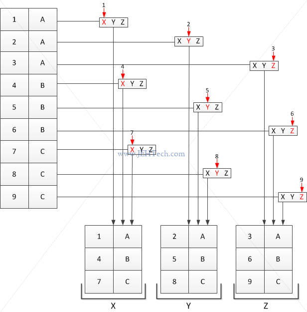
So, as you can see, it is not really a grouping operating. It is really just flinging each ith row into a bucket with the name of the corresponding ith factor variable, and if there are not enough factor variables then they are recycled. That is why it is only acting like a group-by when we pass in a data frame and a row of the data frame as the factor to split on.

Okay, great, but what's the use in this. Well usually we would, instead of splitting a data frame in its entirity, we would split a column we are interesting in calculating some statistics over based on a grouping re another column. In the above example, we might want to find the mean of the column "a" for each of the groups "A", "B" and "C". We would use the following:

> with(x, lapply(split(a, c), mean))
$A
[1] 2

$B
[1] 5

$C
[1] 8

Find some training data at
http://archive.ics.uci.edu/ml/datasets.html.

http://data.gov.uk/data/search.
DATA FRAMES
-----------

x[row, col] with indices or actual names or slices or boolean conditions
  eg x[condition1 & condition2,] -- select only certain rows
  which() returns indices and doesnt return the NAs

sort(x$colname, decreasing=TRUE/FALSE, na.last=TRUE)

x[order(x$colname1, x$colname2, ...),] - order rows so column(s) in order

plyr package for ordering
arrange(dataframe, colname) -asc order
arrange(dataframe, desc(colname)) - same with decreasing order

add row/col
-----------
df$new_col <- ... vector

or use cbind() command - column bind
or
library(plyr)
mutate(df, newvar=...) - adds new col and returns new datafame copy.









TODO: Cross tabs (xtabs)



TEXTUAL FORMATS
---------------
dump() and dput()
saves metadata like column class.
still textual so readable but meta data included
textual data works better in version control software
but not space efficient

y <-data.frame(...)
dput(y) prints to screen
dput(y, "filename.R") saves to file
y2 <- dget("filename.R") loads DF back into Y2

Looks like little bit like object pickling in Python

dget() can only be used on a SINGLE R object.

dump() can be used on multiple objects, which can then be read back using a single 
source() command

eg.
x <- ...
y <- ...
dump(c("x", "y"), file="...") // pass NAMES of objects in
rm(x, y)
source("...")
// restores x and y



CONNECTIONS TO THE OUTSIDE WORLD
--------------------------------
file
gzfile (gzip)
bzfile (bzip2)
url (webpage)

above function open connectsion to a file or a web page

con <-file("foo.txt", "r")
data <- read.csv(con)
close(con)

same as data <- read.csv("foo.txt")

con <- url("http://....")
x <- readLines(con)
// x will be a character vector holding page source 





DATES & TIMES
--------------
	Dates - Date class
	        Stored internally as days since 1-1-1970
	Times - POSIXct or POSIXlt class
	        Stored internallay as seconds since 1-1-1970
	        POSIXct just a large integer
		POSIXlt is a list storing day, week, day of year, month, etc etc

Convert strings to dates using as.Date()
	x <- as.Date("1970-01-02")
	unclass(x) == 1 

Generic functions:
	weekdays() - Give day of the week
	months()   - Gives month name
	quarters() - Gives "Q1", "Q2" ...

x <- Sys.time()
p <- as.POSIXlt(x)
p$sec == ..seconds..

strptime() converts dates to an object
eg
	datestring <- c("January 10, 2013, 10:30")
	x <- strptime(datestring, "%B %d, %Y %H:%M")
	x will be a POSIXlt object

	?strptime for help on function

Normal +,-,<,> etc work on dates

The operators keep track of leap years, leap seconds, daylight savings and timezones
for us automatically :)

LOOP FUNCTIONS
--------------
All implement the Split-Apply-Combine strategy: SPLIT into smaller pieces,
APPLY a function to each piece, COMBINE the results.

lapply() - loop over list and eval func for each element. looping done in C
split() - splits objects into sub-pieces

lappy(list, function_name, ) returns result for every object in the list as a list in the same order. 'function_name' is applies to each element of the list and the return value used for that element in the new list. The  arguments will be passed to your function_name().

lappply() generally uses ANONYMOUS FUNCTIONS.
lapply(x, function(params){...}) 

sapply() - simplifies result of lapply(). Each list might go to vector if every element has length one. If cant figure out the simplification a list is returned.

apply(X, margin, fun,...)
	margin is an int vector indicating which margins should be retained
	fun is func to be applied
	 passed to 'fun'

	the margin refers to the DIMENSION number being used. For a matrix 
1 is rows 2 is columns. 

	So. apply(x,2,mean) would apply mean() to columns of matrix.
	For row/col sums/means use more highly optimized functions for SPEED
	rowSums = apply(x,1,sum)
	colSums = apply(x,2,sum)

	can keep two dims using appy(x, c(1,2,...), ) for multi dim arrays
	or use rowMeans(..., dim=x)


mapply(fun, , MoreArge=NULL, SIMPLIFY=TRUE, USE.NAMES=TRUE)
	Applies a func in parallel over a set of different arguments.

	Eg two lists where element x in list_1 is param of 'fun' and element x in list_2 is second param. this is what mapply helps you do.

	Use to VECTORIZE FUNCTIONS that normally act on scalars.

tapply(x, index, fun, ...) - apply a function over subsets of a vector.
   index is a factor or a list of factors which identifies which group each 
   element of the numeric vector is in.

   e.g.
   x <- c(rnorm(10), runif(10), rnorm(10,1))
   f <- gl(3,10) // creates a factor variable, each one repeated 10 times
     == 1 1 1 1 1 1 1 1 1 1 2 2 2 2 2 2 2 2 2 2 3 3 3 3 3 3 3 3 3 3
        levels: 1 2 3
   tapply(x, f, mean)
   1      2      3
   0.114  0.516  1.246 

   if you dont simply the result you get back a list

   You can subset a matrix to do the equivalent of an SQL GROUP BY:
      with(df, tapply(col1, col2, mean))
   This will group by col1 and take the mean of col2 using that grouping.

split(x, f, drop = false, )
like tapply() it splits x into groups where f identified which group each element of x is in.

common to split() something then apply a function over the groups:
	lapply(splot(x,f), mean) for example

split() can be  used on complex data structures like dataframes.
	e.g. s <- split(dataframe, dataframe$col_name)
	     lapply(s, function(x) snip )

	tip: use sapply(... na.rm=TRUE) 

To split on more than one level, combine factors using interaction():
	x <- rnorm(10)
	f1 <-gl(2,5) # 1 1 1 1 1 2 2 2 2 2, levels 1 2
	f2 <-gl(5,2) # 1 1 2 2 3 3 4 4 5 5, levels 1 2 3 4 5
	interaction(f1,f2) 
#10 levels 1.1 2.1 1.2 2.2 1.3 2.3 1.4 .. 2.5

> f1 <-gl(2,5) # 1 1 1 1 1 2 2 2 2 2, levels 1 2
> f1
 [1] 1 1 1 1 1 2 2 2 2 2
Levels: 1 2
> f2 <-gl(5,2)
> f2
 [1] 1 1 2 2 3 3 4 4 5 5
Levels: 1 2 3 4 5
> interaction(f1,f2) 

1 1 1 1 1 2 2 2 2 2
. . . . . . . . . .
1 1 2 2 3 3 4 4 5 5
  |
  |
       \/
    [1] 1.1 1.1 1.2 1.2 1.3 2.3 2.4 2.4 2.5 2.5
Levels: 1.1 2.1 1.2 2.2 1.3 2.3 1.4 2.4 1.5 2.5
	
NOTE: Although it says there are all those levels it appears it uses the returned array, not the levels themselves which is why it returns missing values for some levels so it has all the levels but not all are used.

split(x, list(f1,f2), drop=TRUE)
$'1.1'
[1] 2.0781323 0.7863726

$'1.2'
[1] -0.7285167  0.1410324

$'1.3'
[1] 0.643741

$'2.3'
[1] -0.7616546

$'2.4'
[1] -0.4612373 -0.6063274

$'2.5'
[1]  0.0106792 -0.5811911


split(drop = TRUE) to drop empty levels


Some useful functions
----------------------
range() returns the minimum an maximum of its argument
unqiue() returns vector with all duplicates removed
grep, grepl, regexpr, gregexpr and regexec search for matches to argument 
pattern within each element of a character vector



DEBUGGING
---------
Return something invisibly: return the value but dont print it use invisible(x).

5 basic functions
traceback()
   prints function call stack
debug()
   flags function for debug mode which lets you step through
      eg
        debug(func)
        func()
        Then drops into browser
        "n" to step through to next instruction
browser()
   suspends execution wherever it is called and puts func into debug mode
trace()
   allos insert debugging code into function at specific places
recover()
   allows modification of the error behabiour so you can browse the function 
   call stack 
      options(error = recover)

R Profiling
-----------

Figure out why things are taking time and suggest strategies for fixing.
Systematic way to examine how much time is being spent in various parts
of your program.

system.time()
-------------
Takes R expression (can be in curley braces) an returns time taken to
do the expression in seconds.

Returns proc_time
   user time    - CPU time 
   elapsed time - "wall clock" time

There are multi-threaded BLAS libaries (ATLAS, ACML, MKL)
Parallel package for parallel processing

http://stackoverflow.com/questions/5688949/what-are-user-and-system-times-measuring

The "user time" is the CPU time charged for the execution of user
instructions of the calling process. The "system time" is the CPU
time charged for execution by the system on behalf of the calling
process.

Rprof()
--------
R must be compiled with profiler support.

Rprof() starts the profiler
DO NOT USE system.time() with Rprof()

summaryRprof() to summarise Rprof() output
   by.total - divide time spent in each function by total time
   by.self  - divide time spend in each function minus time 
              spent in functions above by total time.

Rprof() tacks FUNCTION CALL STACK at regularly sampled intervals

Generate (pseudo) random numbers
---------------------------------
   - rnorn() random normal with mean and stddev
   - dnorm() evaluates standard normal prob density funct at point or 
             vector of points
   - pnorm() eval cumulative distribution function for normal distribution
   - rpois() generate random Poisson with a given rate
   - rbinom() uses binomial distribution

   d for density
   r for random number gen
   p for cummulative distribution
   q for quantile function

Important: use set.seed(<seed>)
           this resets the sequence that will occur.


Random sampling
----------------
THe sample() function draws randomly from a specified set of (scalar)
objects allowing you to sample from arbitrary distributions.

set.seed(...)
sample(1:10, 4)               # without sample replacement
sample(1:10, 4, replace=TRUE) # with sample replacement 
                              # (so can get repeats)

READ DATA FROM WEB (HTTPS)
-------------------------
library(RCurl)
url <- "https://d396qusza40orc.cloudfront.net/getdata%2Fdata%2Fss06hid.csv"
data <- getURL(url, ssl.verifypeer=0L, followlocation=1L)
writeLines(data,'temp.csv')

get binary data using getBinaryURL(...) and the following:
   tf <- tempfile()
   writeBin(con=tf, content)

READ DATA FROM EXCEL
--------------------
library("xlsx")
dat <- read.xlsx(fname, startRow=18, endRow=23, colIndex=7:15)


XML into R
---------------
library(XML)
doc <- xmlTreeParse(url, useInternal=TRUE)
   there is also htmlTreeParse for HTML files!
rootNode <- xmlRoot(doc)
xmlName(rootNode)

xmlName() - element name (w/w.o. namespace prefix)
xmlNamespace()
xmlAttrs() - all attributes
xmlGetAttr() - particular value
xmlValue() - get text content.
xmlChildren(), node[[ i ]], node [[ "el-name" ]]
xmlSApply()
xmlNamespaceDefinitions()

xmlSApply(node, function-to-apply) - recursive by default
or xpathSApply(node, xpath-expression, function-to-apply)


XPath language
/node - top-level node
//node - node at any level
node[@attr-name] - node that has an attribute
named "attr-name"
node[@attr-name='xxx'] - node that has attribute named attr-name with value 'xxx'
node/@x - value of attribute x in node with such attr.


FAST TABLES IN R
-----------------
data.table

Is a child of data.frame but is much FASTER.
Has a different syntax

Create in exactly same way is data.frame


tables() - all data.tables in memory

Subsetting with only one index subsets with ROWS

Subsetting columns very different.
   EXPRESSIONS
   Uses expressions: satements between curley brackets {}
      e.g. dt[, new_col := {some expressions...}

   LISTS
   Or use a list of functions to apply to columns:
      e.g. dt[, list(mean(x), sum(z))]

   ADD NEW COL (very efficiently) with := syntax
      dt[,w:=col-name]
      Adds inplace
      Data tables copied BY REFERENCE so be careful of aliases!
      Create copied explicitly using copy() function

Grouping using 'by=' syntax.
   Special variable .N to count group
      eg. dt[, .N, by=...]

Keys for fast indexing. joins, merges, subsetting, grouping
   e.g. setkey(dt, col-name)

Apparently even faster is
http://www.inside-r.org/packages/cran/data.table/docs/fread


MYSQL
-----
dbCon <- dbConnect(MYSQL(), user="...", host="...", db="...")
allTabls <- dbListTables(dbCon)
result <- dbGetQuery(dbCon, "SQL QUERY STRING")

dbListFields(dbCon, "TABLE NAME") - lists field names in table
dbReadTable(dbCon, "TABLE NAME") - reads the ENTIRE table (caution - size!!)

To select a subset:
   query <- dbSendQuery(dbCon, "SQL STR") - doesn't get the data
   x <- fetch(query, n=number-of-rows) - this gets the data
   dbClearResult(query) - must be done after a query!

dbDisconnect(dbCon) - must be closed!!!! see on.exit() function for safety

http://www.r-bloggers.com/mysql-and-r/


HDF5
----
source("http://bioconductor.org/bioLite.R")
biocLite("rhdf5")

library(hdf5)
f = h5createFile("...")
g = h5createGroup("file-name", "group-name")
h5ls("file-name") - dump out file info

Write data:
   A = matrix(1:10, nr=5, nc=2)
   h5write(A, "filename", "group/path/to/var/spec")

   will automatically write meta data for you too
   attr(A, "somejunk") <- "a value"

See bioconductor notes


FROM WEB
--------

con = url("...")
htmlCode = readLines(con)
close(con) 

htmlCode is just the raw code as one blob.
Alternative use htmlTreeParse() and xpathSApply() etc


creating new variables
=======================

create sequence
----------------
s1 <- seq(min-val, max-val, by=incr-value)
s1 <- seq(min-val, max-val, length=) - has length values
s1 <- seq(along = x) vector of indices for x

create binary vars
--------------------
x <- ifelse(df$col <op> cond, TRUE, FALSE)



create categories
-----------------
apply to quantative variables
x <- cut(df$col, breaks=....) The breaks specifies the boundaries for the groups
   eg cut(df$col1, breaks=quantile(df$col2))

or use library(Hmisc)
   cut2(df$col, g=4) - shortcut for quantiles


reshape data
==============
USE THE reshape2 library
   library(reshape2)

tidy data
   1. every variable its own col
   2. every observation its own row
   3. each table/file to store data about only one kind of observation


melt a dataframe
-----------------
melt(df, id=c(...), measure.vars=c(...))
   create a new df. variables in id list are repeated for each variable in measure.vars
   so that rather than being wide the df becomes thin with a row for each variable with
   ids acting like the index or identifier. Thus is there are 2 items in measure.vars
   there will be 2 occurances of the identifiers in id list.

cast data frame
----------------

using dcast() to summarise a dataset
- - - - - - - - - - - - - - - - - - -
   dcast(df, col-to-group-by ~ col-to-summarise)
      will take col-to-group-by and produce a row for each unique value in that set.
      then it groups by those values and applies, by default, a count to see how many
      instance of col-to-summarise belong to that group.

   if you dont want to count, you can apply any aggregation operation
      dcast(df, col-to-group-by ~ col-to-summarise, mean)


split-apply-combine problems
------------------------------
Notes on this article:
www.r-bloggers.com/a-quick-primer-on-split-apply-combine-problems

Further note by Hadley Wickham

list_by_group <- with(df, split(col-to-count, col-to-group-by))
aggr_by_group  <- sapply(list_by_group, aggregation-function)
   e.g. aggregation-function could be mean()

This can be summarised in one command in these different ways:
   1. with(df, tapply(col-to-count, col-to-group, agrregate-function))
        The tapply() function does an inherent group by operation for you
   2. with(df, by(col-to-count, col-to-group, agrregate-function))
   3. aggregate(col-to-count ~ col-to-group, df, agrregate-function)
  


dplyr package
===============
library(dplyr)

Basic verbs used by package:
   select    - returns a subset of columns of df
   filter    - extract subset of rows
   arrange   - reorder rows
   rename    - rename a column
   mutate    - add new variables or columns. transform existing
   group_by  -
   pipeline  - use %>% to pipe output to next func.
               then funcs won't need the df argument, they get it from the pipeline
   join      - faster but less fully featured than merge(). this can only merge
               on common names, you can spec the cols!
   join_all  - join multple df's. Takes list as argument
   summarise -
 

Format generally:
   new_df<- dplyr-func(df, what-to-do-with-df)


select
------
Can use column names in ranges rather than just indices
  select(df, col-name1:col-name2) - select all columns in this range
  select(df, (-col-name1:col-name2)) - select all columns EXCEPT those in this range


filter
-------
filter(df, col <op> cond)


arrange
-------
   df <- arrange(df, col-name) - order dataset by this column, asc order
   df <- arrange(df, desc(col-name)) - order dataset by this column, desc order


rename
------
   df <- rename(df, col-name-new=col-name-old, ...)  - renames those cols, leaves others as is


mutate
------
transform existing vars or create new ones
   df <- mutate(df, new.col=....) - adds a new column
eg
   df <- mutate(df, new.col=old.col - mean(old.col)) - adds a new column


group_by
---------
   grouped_df <- group_by(df, colname)
   summarise(grouped_df, label1=func(col-name), ....)



merging data
=============
By default merges by columns with common name. Use by.x, by.y to tell it which cols
  by.x is the first df
  by.y is the secon df

  use "all=TRUE" for an outer join


merge(df_x, df_y, by.x=, by.y=, all=)

can also use join in plyr package


Misc
----
remove the original data frame from your workspace with rm("variable-name")
packageVersion("package name") to get the package version


Manipulating Data with dplyr
----------------------------
FIRST, you must load the data into a 'data frame table' 
   data_df_tbl < tbl_df(data_df)

dplyr supplies five 'verbs' that cover most fundamental data manipulation tasks: select(), filter(), arrange(), mutate(), 

and summarize().

dplyr also doesn't print all teh data. to see it all use View() (best done in R Studio)

select(data_df_tbl, colname1, colname2,...) 
   works on COLUMNS
   returns a new df_tbl with only the cols named in the order specified
   given this ordering, select can then allow us to use the range operator ":"
      with column names rather than indices.
      e.g. select(data_df_tbl, colname4:colname6) 
         the order can be reversed as in colname6:colname4 too.

   to specify column to dump rather than keep use a minus "-".
   eg. select(data_df_tbl, -colname1) gives all columns except colname1
   eg. select(data_df_tbl, -(colname1:cn3)) gives all columns except those in the range specified
                                            note the range must be enclosed in brackets to negate 
                                            the entire range (rather than just the start element)
   
   Special select functions (from helpfile):
      - starts_with(x, ignore.case = TRUE): names starts with x
      - ends_with(x, ignore.case = TRUE): names ends in x
      - contains(x, ignore.case = TRUE): selects all variables whose name contains x
      - matches(x, ignore.case = TRUE): selects all variables whose name matches the regular expression x
      - num_range("x", 1:5, width = 2): selects all variables (numerically) from x01 to x05.
      - one_of("x", "y", "z"): selects variables provided in a character vector.
      - everything(): selects all variables.


filter(data_df_tbl, boolean-vector-selecting-rows, boolean-vector... )
   works on ROWS (the bool vectors are ANDed. To OR use "|" not "," )
   eg. to select rows where a column value is not NA use:
      filter(data_df_tbl, !is.na(col-name))


arrange()
   orders the ROWS of a dataset according to a particular variable.
   eg to order ascending
      arrange(data_df_tbl, colname)
   eg to order descending
      arrange(data_df_tbl, desc(colname))

   Can arrange based on multiple variables, sort my left most first, then next continuing right.

mutate()
   Creates a new variable based on the value of one or more variables already in a dataset. 
   eg.  mutate(data_df_tbl, col_new = someFunc(col_existing))

   Can also use values created in col_new's to the left, in col_new's to the right
   eg.  mutate(data_df_tbl, col_new = someFunc(col_existing), col_new2 = col_new * 0.25)

summarize() 
   collapses the dataset to a single row, especially when data is grouped
   eg summarise(data_df_tbl, some-summary=func(col-name))
   most useful with the group_by() verb

group_by()
   When using summarize() on a table that has been group_by()'ed it will
   return the summary functions for EACH group rather than just one value :)

merge()
   By default merges by columns with common name. Use by.x, by.y to tell it which cols
     by.x is the first df
     by.y is the secon df
   
     use "all=TRUE" for an outer join
   
   
   merge(df_x, df_y, by.x="col1", by.y="col2", all=)
                          ^
                          Note col names are in quotes
                          otherwise you get
                          Error in fix.by(by.x, x) : object 'col1' not found


Some special functions:
   - n()
     The number of observations in the current group. (ie. num rows)
     This function is implemented special for each data source and can only 
     be used from within summarise, mutate and filter.

   - n_distinct()
     Efficiently count the number of unique values in a vector
     Faster and more concise equivalent of length(unique(x))


quantiles
----------
| We need to know the value of 'count' that splits the data into the top 1% and bottom 99% of packages based on total 

downloads. In statistics, this is called the
| 0.99, or 99%, sample quantile. Use quantile(pack_sum$count, probs = 0.99) to determine this number.

> quantile(pack_sum$count, probs = 0.99)



tidying data with tydr
-----------------------
library(tidyr)
http://vita.had.co.nz/papers/tidy-data.pdf

gather()
   Use gather() when you notice that you have columns that are not variables
   Looking at the example from the help file

   > # From http://stackoverflow.com/questions/1181060
   > stocks < data.frame(
   +   time = as.Date('2009-01-01') + 0:9,
   +   X = rnorm(10, 0, 1),
   +   Y = rnorm(10, 0, 2),
   +   Z = rnorm(10, 0, 4)
   + )
   > head(stocks)
           time          X          Y         Z
   1 2009-01-01  0.3269115  0.7445885  6.257515
   2 2009-01-02 -1.5729436 -3.3722382  2.050222
   3 2009-01-03 -0.5257739 -1.2664309 -5.498621
   4 2009-01-04 -1.4181633 -0.2352554  2.338179
   5 2009-01-05 -0.6081603 -2.1707088  2.099759
   6 2009-01-06  0.8347829  2.5455941  9.737100

   > x = gather(stocks, stock, price, -time)
   > head(x)
           time stock      price
   1 2009-01-01     X  0.3269115
   2 2009-01-02     X -1.5729436
   3 2009-01-03     X -0.5257739
   4 2009-01-04     X -1.4181633
   5 2009-01-05     X -0.6081603
   6 2009-01-06     X  0.8347829

   
   What have we done here? In our original data set we had 3 columns. Each represented
   the price of a stock. We want to have one column for the stock type and one column
   for the price of that stock.

   Why do we want this? This is one of the principles of "tidy data". (see
   http://vita.had.co.nz/papers/tidy-data.pdf). Really what we are discussing
   is type-of-stock and price-of-stock at a time. Therefore there are 3 variables
   and each column should be a variable. As it stands the dataset columns
   represent the type-of-stock variable split over many columns. This isn't always
   a bad thing, as the article discusses, but it can be tidied to just have the
   variables as columns: time, stock and price. This is called "melting" the dataset.


   So... gather(stocks, stock, price, -time)
   The data argument, stocks, is the name of the original dataset.
   The key/value arguments, stock and price, give the column names for our new tidy
      dataset. Stock is the key, because it specifies all the column names, X, Y, and 
      Z are to be collected under this new variable... they become like keys in a
      DB table. The value argument is the values of these columns that will be matched
      to the key.
   -time excludes time from the melt, because it is already a variable 

separate() 
   separate one column into multiple columns

spread()
   Spread a key-value pair across multiple columns.

extract_numeric()
   Easy way to just get the numbers out of a string. eg if you have
   a numerical identified with a common textual prefix.



STANDARD FILE DOWNLOAD STUFF
----------------------------

if(!file.exists(your-dir-name)) { dir.create(your-dir-name) }
url < "https://....."
download.file(url, destfile=your-file-name, method="curl")
data < read.csv(your-file-name)

On windows, however, I seem to need to do this
   library(Rcurl)
   if(!file.exists(your-dir-name)) { dir.create(your-dir-name) }
   url < "https://....."
   writeLines(getURL(url, ssl.verifypeer=0L, followlocation=1L), your-file-name)
   data < read.csv(your-file-name)


EDITING TEXT VARIABLES
----------------------
tolower() - returns all lowercase
toupper() - returns all uppercase
strsplit(string, seperator). Remember to escape a character you need double backslash. eg. "\\."
sub(str-to-search-for, replacement-str, string) - replace first instance only
gsub() - replace all instances
grep(regexp, str, value=T/F) - returns indices
grepl() - returns boolean mask vector

library(stringr)
   nchar(str) - number of chacacters
   substr(str, start-index, end-index). Indices from 1 and are inclusive
   paste(str1, str2, sep=" ")
   str_trim() - trim off spaces at start or end.

Names of variables
   * All lower case when possible
   * Descriptive as possible
   * Not duplicated
   * Not have underscores, dots or whitespace


Working with dates
-------------------
date() - returns string od date and time
Sys.Date() - returns a Date object. Can reformat using format()
             Date objects can be subtracted, added etc
format(Sys.Date(), "format-string")
    where format-string is like a prinf expression with these special placeholders
       %d = day as number (0-31)
       %a = abbreviated week day name
       %A = full week day name
       %m = month number (two digits)
       %b = abbreviated month
       %B = unabbreviated month
       %y = 2 digit year
       %Y = 4 digit year

as.Date(char-vector, format-string) turns character vectors into dates
weekdays(date-obj) returns the week day as a string
months(date-obj) returns the logn month name as a string
julian(date-obj) returns number of days since epoch (1st Jan 1970)

library(lubridate)
   Easy date manipulation
   Instead of as.Date(..., "format") you can use...
      ymd(...) which will search for year, month, day in *all* feasible formats
      mdy(...) will search for month, day, year in *all* feasible formats
      ymd_hms(...) date and time
      and so on...
   The functions also accept the timezone using the tz argument to the functions.
   wday(..., label=TRUE) == weekdays() in lubridate



data resources
---------------
http://data.un.org     - united nations
http://www.ons.gov.uk/ons/index.html- uk office for national statistics
https://open-data.europa.eu - european data on EU
http://www.data.gov    - usa gov
http://www.data.gov/opendatasites <--- look here
http://www.data.gov.uk - uk data site
http://www.gapminder.org
http://www.asdfree.com - help on usa surverys
http://www.infochimps.com/marketplace
http://www.kaggle.com
http://data.worldbank.org

Plotting in R
====================================================================

boxplot(df$col, col="blue", breaks=100)
	breaks is the number of bars (or buckets)
hist(df$col, col="green")
rug(df$col) - puts a "rug" under the histogram


abline(h=num) - draw a horizontal line
abline(v=num, col="red", lwd=2) - draw a vertical line
	lwd is line width

barplot()


base plotting system
	- the oldest
	start with blank canvas and add things to it one by one




plot(x,y) or hist(x) launches the graphics device
plot() is generic... it can behave diff depending on the data passed to it.
?par for base graphipcs system parameters

eg with(df, plot(col1, col2))

key plotting parms
	pch  - the polotting symbol
	       a number representing a symbol types.
	       try example(points) on the command line
	lty  - the line type
	lwd  - line width as integer multuple
	col  - colour
	xlab - the label for x axis
	ylab - the label for y axis
	legend

par() used for GLOBAL graphics parameters:
	las - orientation of axis labels on plot
	bg - background coloour
	mar - margine size
	      margine 1 is the bottom, then rotate CW for 2, 3, 4
	oma - outer margin size
	mfrow - # plots per row, col (filled row wise)
	mfcol - # plots per row, col (filled col wise)

base plotting functions
	plot() - scatter plot
	lines() - adds lines to a plot
	points() adds points to a plot
	text() add text labels to plot at specific x,y corrds
	title - add annotations to x, y axis labels, title, subtitle etc
	mtext - add arbirary text to margins
	axis - add axis ticks/labels

multiple base plots:
	par(mfrow = c(rows, vols))
	with(your-dataframe, {
		plot(some data in first plot)
		plot(plot some data in second plot)
	})


To setup plot without plotting anothing
plot(x,y type="n")
             ^^^^ make a plot except for the data
Then you can plot the data sets one by one.

Launch screen device
	quartz() on mac
	windows() on windows
	x11() on linux

?Devices for list of devices available

eg for pdf
	pdf(file = "...")
	...plotting....
	dev.off() ## Close the graphics device!

Vector formats:
	pdf
	svg
	wim.metafile
	postscript

Not so great with many individual points (file size)
Resize well.

http://research.stowers-institute.org/mcm/plotlayout.pdf

Bitmaps:
	png. 
	jpeg. lossy compression
	tiff. lossless compression
Generally dont resize well
good for many many points.


Many devices
--------------
Can only plot to the *active* device
dev.cur() 0 returns graphics device num >=2
dev.set(<int>) change the active device

dev.copy
dev.copy2pdf - copy active plot to new plot
E.g:
	...plot...
	dev.copy(png, file = "filename.png")
	dev.off()

hierachical clustering
=======================
- what is close/
- how do we group things
- How do we visualise the grouping
- How do we interpret the grouping

Agglomerative approach:
- Find closest two things - requires knowing what "closest" means
   - continuous - euclidean sqrt( (x1-x2)^2 + (y1-y2)^2) - extends to hi D probs
   - Continuous - correlation similarity
   - Manhatten - total(x) + total(y)
- Put them together - a "merge"
   - How do we merge?
   - What represents the new location - "average linkage"  - ave of x and y coords - center of grav.
                                      - "complete linkage" - take furtherst two points of clusters as dist.
- Repeat
- A tree results shoing the ordering of how things were grouped.

To simulate a simple 2D dataset:
   set.seed(1234)
   par(mar = c(0, 0, 0, 0))
   x <- rnorm(12, mean = rep(1:3, each=4), sd=0.2)
   y<- rnorm(12, mean = rep(c(1, 2, 1), each = 4), sd = 0.2)
   plot(x,y, col = "blue", pch=19, cex=2)
   text(x+0.1, y+0.1, labels=as.character(1:12))

   df <- data.frame(x = x, y = y)
   distxy <- dist(df) # cacls dist between all different rows/cols combos in df.
   hCllust <- hclust(distxy)
   plot(hCllust)


heatmap() for looking at matrix data - does a hierachical cluster of rows and cols of the matrix
   rows are like observations
   cols are like sets of observations

   organises the rows and columns of the table to visualise groups or blocks within the table




k-means clustering
===================
K-means is NOT deterministic. If you run multiple times but resulst vary to much the alg might
not be stable w.r.t to your data!

It is a partitioning approach
   - Define #groups you would
   - Get "centroids" for each cluster
   - Assigned to closests centroid
   - Recalc centroids and iterate

   set.seed(1234)
   par(mar = c(0, 0, 0, 0))
   x <- rnorm(12, mean = rep(1:3, each=4), sd=0.2)
   y <- rnorm(12, mean = rep(c(1, 2, 1), each = 4), sd = 0.2)
   plot(x,y, col = "blue", pch=19, cex=2)
   text(x+0.1, y+0.1, labels=as.character(1:12))

   df <- data.frame(x = x, y = y)
   kmeansObj <- kmeans(df, centers = 3)
   par(mar = rep(0.2, 4))
   plot(x, y, col = kmeansObj$cluster, pch=19, cex=2)
   points(kmeansObj$centers, col = 1:3, pch=3, cex=3, lwd=3)

Lattice plotting system
=========================

- Good for high density plots
- package(lattice)
   - xyplot     - scatter plots
   - bwplot     - box plots
   - histogram
   - stripplot
   - dotplot
   - splom      - scatter plot matrix. like pairs() in base plot
   - levelplot  - image data
- Everything (i.e. entire plot) is done in a single function call
- lattice functions return calls called "trellis". this must
  be printed to the device to dislplay it on. Auto-prints for
  desktop display

xyplot
xplot(y ~ x | , data)
   y is the y data
   x is the x data
   condition vars (optional). they are factor variables
      and conditioning on them creates n graphs for each
      level of the condition var
   data is the dataframe

   eg 
      library(datasets)
      library(lattice)
      airqual <- transform(airquality, Month=factor(Month))
      xyplot(Ozone ~ Wind | Month, data = airqual, layoutc=c(5,1))



panel functions
   Each panel represents a subset of the data defined by the
   conditioning variable supplied

   xyplot(y ~ x | f, panel = function(x,y, ...) {
      panel.xyplot(x, y, ...)
      panel.abline(h=median(y), lty=2)
   })

   By giving the panel function we specify how each 
   panel is to be drawn. Each panel in this case does
   an xyplot, but also does a horizonal line at the data
   median. Note: data for each panel is different we're just
   saying what is to be done with the data on each panel.

   panel.lmline() for least regression line





ggplot plotting system
=======================

Grammar of Graphics by Leland Wilkinson
Built on the grid graphics system. 

qplot()
--------
Works like the plot() function of the base system
data must always come from a dataframe
factors are used to indicate *subsets* of the data

eg qplot(x, y, data=dataframe) where x and y are column 
names in dataframe

to highlight subgroups use qplot(x,y,data=df, color=z) where
z is another column inthe dataframe

to add smoother do
   qplot(x,y,data=df, geom=c("point", "smooth"))

to do histogram
   qplot(x, data=df, fill=z) here fill is like color
   qplot(x, data=df, geom="density") for a desity smooth of hist

to do panels you use facets
   qplot(x,y, data=df, facets=.~z) or
   qplot(x,y, data=df, facets=z~.) 
   it is rows~cols and the "dot" means wildcard

ggplot() 
---------

Plots built up in layers
   - plot data
   - overlay summary
   - add regressions etc

Basic ggplot:
   g <- ggplot(dataframe, aes(x, y[, color=z]))
                          ^^^
                          the aesthetics (cols to be plotted)

   So far there are no layers on the plot - nothing to specify
   how to draw the plot

   So we need to add this to the plot...

   p <- g + geom_point() ## adds "how to draw" information
   print(p) ## display (or use autoprinting)

   or use geom_line()

   Add a smoother
   g + geom_point() + geom_smooth(method="...")
 
   Add a facet grid
   g + geom_point + facet_grid(. ~ z) + ....
                               ^^^^^^
                               works the same as qplot

   To annotate the plots use
   xlab(), ylab(), labs(), ggtitle()
      eg labs(title="...", x="...", y="...")
   theme()
      theme_gray(), theme_bw() some standard appearances

Aesthetics options
   - color=...
   - size=...
   - alpha=..

The smoother.
   - size=
   - linetype=
   - method=..
   - se=...


Note: ylim() will FILTER the data to filter out things outside
      limits. To keep outliers use coord_cartesian(ylim=())

Categorise on continuos ver:
   To categorize continuous variables use CUT() function!
   Can use quantile() function to get some reasonable
      cut points