1. Excel's VLOOKUP() function.
2. Excel's MATCH() function.

https://stackoverflow.com/questions/5603822/using-relative-positions-in-excel-formulas
https://superuser.com/questions/316239/how-to-get-the-current-column-name-in-excel

The Goal Of Table Lookup

Download the Excel example here.

Had wanted to index a matrix, or table, but not using the row and column numerical indices but using row and column labels. Lets take a look at a little toy example. I have a matrix of students names and their score for a set of subjects in the following excel spreadhseet:

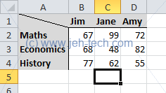
So why index the table using names? Because I want the user to select a row and column entry from a list and be returned the result from the table... I want the user to say "give me Jim's score for Maths" and not have to know that Jim is column 1 of the table and that maths is row 1 of the table:

Creating Drop Down Lists In Cells

So... In another sheet I will have two drop down lists to select a row and select a column:

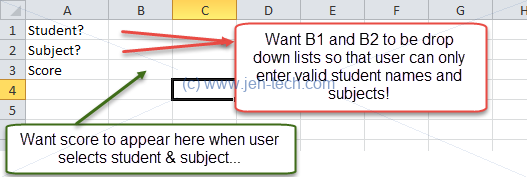
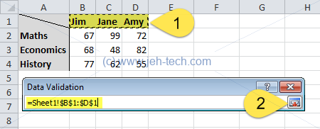
So we need B1 to be a drop down list with the student names from our table and B2 to be a drop down list with the subject titles from our table. To accomplish this we do the following (also shown in the image below)...

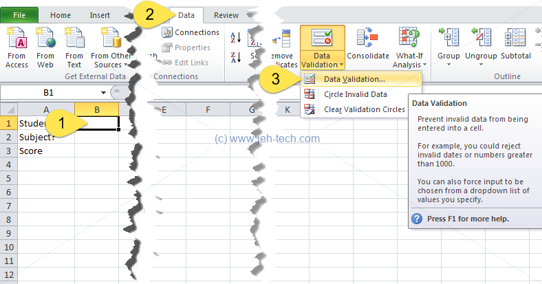
1. Select the B1 cell and then
2. Select the "Data" tab in the ribbon and
3. Drop down the "Data Validation" menu and click on "Data Validation".

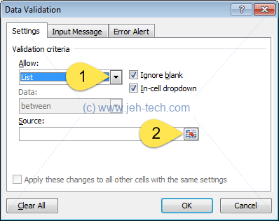
Having done this, the Data Validation dialog will show. This will allow us to restrict the data that can be entered into this cell. We want to

1. Restrict the user input to values in a drop down list so we must select "List" in the "Allow:" field,
2. Select which values appear in our drop down. For that you click on the little icon to the right of the "Source:" input box ().

This is shown in the image below:

Having clicked the data select box () you must then select, from the table in your excel worksheet, the row containing the student names. This is shown below (selected cells highlighted in yellow):

Once you have selected the student names click the "finish" button () to go back to the Data Validation dialog, as shown below.

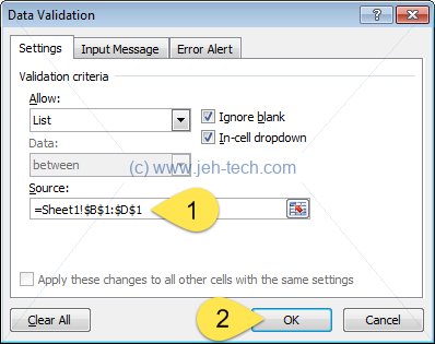
1. You will notice that the range you selected is now in the "Source:" field.
2. Lastly click OK.

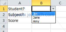
Now you will see in your spreadsheet that cell B1, where we want the user to enter the student name is a drop down list containing all the student names from our matrix. Now the user is constrained to entering only the available names, which is what we wanted.

Exactly the same process needs to be repeated for the test names to create a dropdown in the cell B2. This time when you select the list contents you will select the row labels of the matrix. This is summarised in the image below:

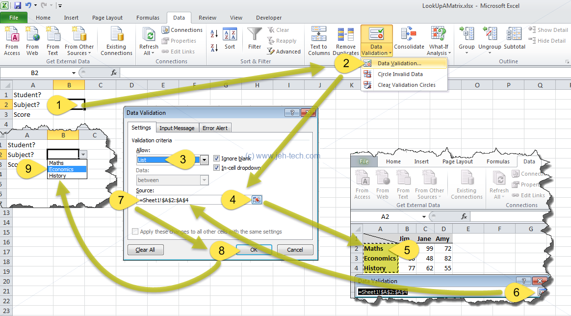
1. Select the cell B2,
2. Select the "Data" tab on the ribbon and select "Data Validation.." from the "Data Validation" drop down icon so that the data validation dialog displays,
3. Select "List" from the "Allow:" field,
4. Click the data select box (),
5. Navigate to the worksheet containing the table and select the row labels for the subject names,
6. Select the finish button (),
7. The range selected appears back in the data validation dialog,
8. Click OK,
9. Done: the result is that cell B2 is now a drop down list containing the test names from the table.

Looking Up A Table

The user is now able to tell us what student and what subject she wants the test score for. Now we need to lookup the table using this information.

As far as I know, Excel doesn't have a function that will directly do this for us, but it does have a table lookup function called VLOOKUP() that will look up values in a table based on a value found in the index row. This function falls short in that to select the column an integer column number must be used. In order to go from column heading to column number we will use another function, MATCH().

Looking Up A Table By Row

VLOOKUP() will look for a value in the first column of a table. Thus the "key" that you are using has to be in the left most column of your table. Given how we've laid out the table, we're ok.

VLOOKUP() works as follows:
VLOOKUP(value, table, column, search type)

1. value is the value, in the left most column of the table, that you want to find, i.e., index your table rows by,
2. table is the rectangular block of cells that constitute your table,
3. column is the column that you want to look up. The column in the row that contained value is the value that the function will return.
4. search type specifies whether your do an exact search (TRUE), where the function will search all cells in the first column for an exact value, or non-exact (FALSE) where the data in the first column of your table must be sorted and the function will return the closest match.

This is shown pictorially in the image below...

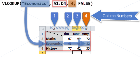
In the above example we are looking for "Economics" in the table (red border). VLOOKUP finds economics in row 3. It then goes along row 3, to column 4 (which we also specified in the function call - the orange highlight) in the table and returns the value in that cell.

Okay, so now we can look up our table by row. We would simply place the string "Economics" in our function call with the cell reference of the cell that contains the user entered value... in the case of this example, cell B2. Thus, the function now becomes VLOOKUP(B2, A1:D4, 4, FALSE).

This is great but we still cannot find the score for any student. Currently we hav a fixed column index of 4, which will look up scores for Amy only...

Finding Column Index From Heading

Cell B1 lets the user pick a student. The question is, how do we go from the students name to the column number in our table for that student? Enter the MATCH() function.

The MATCH() function will search for an item in a list and return the position of the item in the list as a number. The numbering start from 1.

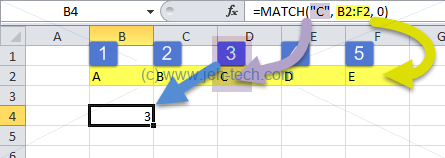
The image above shows an example of how MATCH() works. The yellow highlight shows the row of cells we have used as our array. The blue boxed numbers indicate the numerical positions of each of the values in the array: each cell acts as an element of the array. We have told MATCH() to find the value "C" in our array and return its position, which you can see it does: 3 is returned.

Bringing It Together!

So, we're getting there! Now, to tie this to our example in stead of searching for "C" we would search for the value contained in cell B1. Thus to get from student name to column number we want to use MATCH(B1, A1:D1, 0).

But wait?! Why is A1 in our array?! Cell A1 is empty, but we want this so that the first student name has an index of 2 in our array, as this is the column number for the first student as far as our VLOOKUP() is concerned.

Thus, pluggin this into our VLOOKUP(), the equation for the result cell becomes =VLOOKUP(B2,'Data Matrix'!A1:D4,MATCH(B1,'Data Matrix'!A1:D1,0), FALSE). Download the completed Excel example here.

Wanted to count number of tests that occurred on a specific date. Ans: Create a column with formula as follows.

=IF(F2=DATEVALUE("16/5/2016"),1,0)

Note the use of the DATEVALUE function. Then just sum the column.

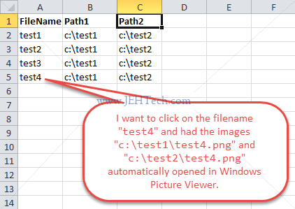
I had a spreadsheet with a set of results. Column A has a filename, column B has a path to a file as named in column A, and column C has a different path to a file as named in column A. I want to click the file name and then open two images: pathInColumn(B) + a and pathInColumn(C) + a. The image below demonstrates this a little more clearly...

To accomplish this I had a bit of a Google and the following is based on these two links.

• VBAExpress: How to open a file with Windows Photo Viewer, answer by user "mdmackillop".
• How to Run an Event in MS Excel If a Cell Is Selected.
• MS Excel Range Object.

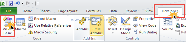
To do this, first save your spreadsheet as a macro-enabled spreadsheet. It will have a .xlsm extension. Load the VBA console from the developer tab.

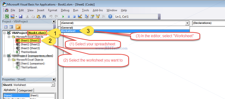
In the VBA editor, in the Project explorer view on the left hand side of the window, select the VBA project for you workbook and drill down to select the worksheet you wish to catch cell selection events for. Double click the work sheet and an editor window is display. In the editor window, select from the top left drop down box "Worksheet". This is shown in the image below...

Once you have selected "Worksheet" the editor will automatically fill in a template for the Worksheet_SelectionChange event. This function is called every time a new cell receives focus. The parameter Target is an MS Excel range object that can be used to find out which cell(s) have been selected by the user.

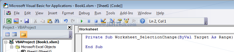
Now that we have the shell of the function, we need to fill it in. Use the code below:

Private Sub Worksheet_SelectionChange(ByVal Target As Range)
    Dim fname1 As String
    Dim fname2 As String
    If Intersect(Range("A1:A1"), Target) Is Nothing Then
        If Not Intersect(Range("A:A"), Target) Is Nothing Then
            If Target.Count = 1 And Not IsEmpty(Target.Value) Then
                fname1 = Target.Cells(1, 2) + "\" + Target.Value + ".png"
                fname2 = Target.Cells(1, 2) + "\" + Target.Value + ".png"

                ActiveWorkbook.FollowHyperlink "file://" + fname1
                ActiveWorkbook.FollowHyperlink "file://" + fname2
            End If
        End If
    End If
End Sub

The first If statement makes sure that the selection is not in the first row of column A as this is our table header. The function Intersect() checks if the range A1:A1 which is our header row is part of the range defined by Target which is the cells that the user has selected.

And so on...