https://stackoverflow.com/questions/28935983/preprocessing-image-for-tesseract-ocr-with-opencv
https://www.pyimagesearch.com/2017/07/17/credit-card-ocr-with-opencv-and-python/
http://citeseerx.ist.psu.edu/viewdoc/download;jsessionid=E6122958EB8D16F13E0EEC460D6207E5?doi=10.1.1.308.445&rep=rep1&type=pdf
https://www.learnopencv.com/hand-keypoint-detection-using-deep-learning-and-opencv
https://www.learnopencv.com/deep-learning-based-human-pose-estimation-using-opencv-cpp-python

Read/Write An Image

References:

• Getting Started with Images, OpenCV docs.
• Extracting a region from an image using slicing in Python, OpenCV. StackOverflow.com

import cv2
myImage = cv2.imread('/path/to/img', ?)  # ? is cv2.IMREAD_COLOR - Load colour but NO transparency
                                         #      cv2.IMREAD_GRAYSCALE - Greyscales image
                                         #      cv2.IMREAD_UNCHANGED - Load colour and transperency
print(type(myImage))                     # Prints <class 'numpy.ndarray'>
cv2.imshow('A Window Title', myImage)    # Displays an image in the specified window.
key = cv2.waitKey(delay=0) & 0xFF        # Param delay waits in milliseconds, 0 forever.
                                         # Returns ASCII code of key pressed.
                                         # And with 0xFF required for 64-bit machines
cv2.imwrite('/path/to/img/cpy', myImage) # Write a copy of the image
cv2.destroyAllWindows()                  # Destroys all of the opened HighGUI windows.

Note that OpenCV uses BGR (Blue, Green, Red) so, if you load a colour image the array dimensions will be (width, heigh, channel), where channel 0 is blue, 1 is green and 2 is red.

You can plot images in Matplotlib too, but because OpenCV use BGR and not RGB, you have to convert images so that they will display correctly. The following is a copy of the code from the referenced SO thread with a few modifications:

import cv2
import numpy as np
import matplotlib.pyplot as plt

# Open your image - an array of width x height x 3-channels
img = cv2.imread('/path/to/img')

# Split out the colour components into their own width x height arrays
b,g,r = cv2.split(img)

# Create a new array that orders the components as RGB
img2 = cv2.merge([r,g,b])

# Create a visual comparison of how a raw OpenCV image array (BGR) would plot vs
# how the RGB image array plots in Matplotlib.
plt.subplot(121);plt.imshow(img)  # expect distorted color
plt.subplot(122);plt.imshow(img2) # expect true color
plt.show()

# Show the difference whe OpenCV displays the image...
cv2.imshow('bgr image',img)  # expect true color
cv2.imshow('rgb image',img2) # expect distorted color
cv2.waitKey(0)
cv2.destroyAllWindows()

The above is demonstrates how the image arrays are stored. However, it is a lot quicker and neater to use cv2.cvtColor() to change colour spaces. As suggested on the referenced SO thread:

img2 = cv2.cvtColor(img, cv2.COLOR_BGR2RGB)

Prefer the above :)

Colour Spaces

You can convert between colour spaces using cv2.cvtColor:

cv2.cvtColor(img, cv2.COLOR_BGR2RGB)   # Go from BGR to RGB
cv2.cvtColor(img, cv2.COLOR_BGR2GRAY)  # Go from BGR to grayscale
cv2.cvtColor(img, cv2.COLOR_BGR2HSV)   # Go from BGR to HSV
cv2.cvtColor(img, cv2.COLOR_BGR2YCrCb) # Go from BGR to luma-chroma (TCC)

There are an absolute ton of conversions available to and from BGR, see the OpenCV docs for all of them!

References:

• Image Thresholding, OpenCV docs.
• Segmentation methods in image processing and analysis, MathWorks.
• Chapter 3: Binary Image Analysis, Computer Vision by Linda Shapiro and Geoarge Stockman.
• Image segmentation.

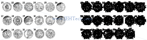
Image segmentation involves grouping the pixels of an image into meaningful sets. For example, lets say we want to count coins on a table. We can take an arial picture of the table and then segment the image into pixels that are part of a coin and those that are not. Then by "globbing" the pixels forming coins, we can count the number of coins.

Thresholding Methods

Thresholding involves converting a grayscale image into a binary (black & white image). This is done by selecting a value. All pixel intensities below this value are made black and everything else white.

The assumptions are that intensity values are different in different regions, thus allowing us to distinguish objects by intensity, and that within each region the intensity values are similar, thus allowing us to "map" the extent of an object.

Simple Thresholding

B&W is useful for a couple of reasons. Firstly it cheap it terms of storage and the complexity of computation over each pixel. Secondly, to detect boundaries etc of objects it can be useful to use B&W and then use algorithms like connected-components to group pixels into objects so that we can say, count or label them.

The most basic thresholding we can do is to pick a pixel intensity ourself and just threshold on it. A very simple way of doing this is shown below (don't ever do it like this!)

import cv2
import matplotlib.pyplot as pl

# Read in the image as gray scale
myImage = cv2.imread('rare-coins.jpg', cv2.IMREAD_GRAYSCALE)

# myImage is just a numpy array so we can use all the numpy maths/logic/array-indexing.
# We create a mask to select all white pixels and make anything non-white black.
blackPixels = myImage < 255
whitePixels = ~blackPixels

# Display the gray scale image
fig, axs = pl.subplots(ncols=2)
axs[0].axis('off') # Hide axis ticks
axs[0].imshow(cv2.cvtColor(myImage, cv2.COLOR_GRAY2RGB))

# Apply our masks and binarise the image before displaying the result
myImage[blackPixels] = 0
myImage[whitePixels] = 255
axs[1].axis('off')  # Hide axis ticks
axs[1].imshow(cv2.cvtColor(myImage, cv2.COLOR_GRAY2RGB))

fig.show()
pl.show()

The result of this is pretty ugly, but here it is. On the left is the original image and on the right the thresholded image.

This pretty niave method can be done much more succinctly using OpenCV's function cv2.threshold() to replace the masking and setting we did using the numpy indexing:

# All pixels with intensity <=254 are made black, the rest white.
ret, myImage = cv2.threshold(myImage, 254, 255, cv2.THRESH_BINARY)
axs[1].axis('off')
axs[1].imshow(cv2.cvtColor(myImage, cv2.COLOR_GRAY2RGB))

The cv2.threshold() function has various threholding options like cv2.THRESH_BINARY.

But, choosing an intensity to threshold on, as done above, is extremely manual. The intensity that was good for the coins, for example, may not be good for a nature scene where we want to seperate the birds from the sky. We'd have to manualy examine each image to decide on an approriate threshold which is resource intensive. Or, perhaps we are seperating animals from their environment: where one animal is in shade and another not, a single threshold value may allow us only to dected one and not the other in the same image!

Local or Dynamic Thresholding

The problem with simple thresholding is that the same intensity value is used both within one image and possible required adjustment, not only within that single image, but across all the images we wish to anaylse.

Dynamic thresholding solves this problem by allowing the threshold value to vary within an image based on some algorithmic properties, thus meaning the human, resource intensive element can be removed.

Some dynamic thresholding methods include:

• P-tile thresholding,
• Optimal thresholding,
• Mixture modelling,
• Adaptive thresholding,
• Clustering: K-means & Otsu’s method.

In OpenCV, to perform dynamic thresholding we use the cv2.adaptiveThreshold() method. Often when thresholding it is useful to apply some kind of blur or smoothing filter to the image to reduce noise. See cv2.medianBlur() or cv2.GaussianBlur() for example.

The Python API is:

cv2.adaptiveThreshold(src, maxValue, adaptiveMethod, thresholdType, blockSize, C[, dst])

Where the more important params are:

maxValue	is the intensity given to pixels for which the local threshold condition is satisfied.
adaptiveMethod	is the thresholding algorithm to use, either ADAPTIVE_THRESH_MEAN_C or ADAPTIVE_THRESH_GAUSSIAN_.
thresholdType	is the threshold type, either THRESH_BINARY or THRESH_BINARY_INV.
blockSize	is the size of a pixel neighborhood that is used to calculate a threshold.

TODO, some more examples and explanations...

References:

• Image Gradients, David Jacobs, Univeristy of Maryland.
• Image Gradients, OpenCV-Python Tutorials.
• Sobel Operator, Wikipedia.

David Jacobs notes introduce the subject perfectly:

The gradient of an image measures how it is changing. It provides two pieces of information. The magnitude of the gradient tells us how quickly the image is changing, while the direction of the gradient tells us the direction in which the image is changing most rapidly.

Sobel kernels are used to calculate the differential of the image are:

$$ G_x = \left[ \begin{matrix} 1 & 0 & -1 \\ 2 & 0 & -2 \\ 1 & 0 & -1 \\ \end{matrix} \right] $$

$$ G_y = \left[ \begin{matrix} 1 & 2 & 1 \\ 0 & 0 & 0 \\ -1 & -2 & -1 \\ \end{matrix} \right] $$

So we could plug some numbers in and see what the vertical edge kernel does...

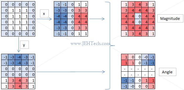
We can see that it has detected and emphasised edges in the image and set to zero areas of the image that do not change. We can also see that there is a change in sign depending on which way the gradient goes. So that's an intuitive look at what the gradient calculation is doing and how it could even be used as an edge detector.

To calculate the gradient magnitude and direction for each pixel we use the following formulas: $$ G = \sqrt{G_x^2 + G_y^2} $$ $$ \Theta = \arctan\left(\frac{G_y}{G_x}\right) $$ We can see this in the image above too. What we can see there, in the magnitude grid that the edge detection has essensitally found the edge around the square.

TODO: Don't understand the angle grid... should have the middle edges I'd have thought... need to understand better :'(

References:

• Canny Edge Detection, OpenCV-Python Tutorials.
• Image Edge Detection: Sobel and Laplacian, K Hong.

Tips

Once again, taking a blur of the image, try cv2.GaussianBlur(), can help reduce noise and improve the performance of the algorithms.

Canny Edge Detection

Use the function cv2.Canny(). It uses the following very high level process...

Gaussian filter
v
Find intensity gradients
v
Apply non-maximum suppression
v
Apply double threshold to determine potential edges
v
Track edge by hysteresis

Sobel Edge Detection

Use the function cv2.Sobel().

Laplacian Edge Detection

use the function cv2.Laplacian().

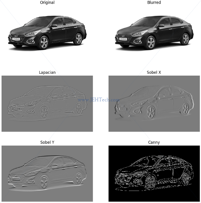
Comparing Canny vs Sobel vs Laplacian

The following snippet, construction based heavily on the references, tries to compare the different techniques...

import cv2
import numpy as np
from matplotlib import pyplot as plt

orignalImg = cv2.cvtColor(cv2.imread('hyundai-verna.jpg',), cv2.COLOR_BGR2GRAY)
gaussImg = cv2.GaussianBlur(orignalImg, (5, 5), 0)

fig, axs = plt.subplots(nrows = 3, ncols=2)
imgList = [(axs[0][0], "Original", orignalImg),
           (axs[0][1], "Blurred", gaussImg),
           (axs[1][0], "Lapacian", cv2.Laplacian(gaussImg, cv2.CV_64F)),
           (axs[1][1], "Sobel X", cv2.Sobel(gaussImg, cv2.CV_64F, dx=1, dy=0, ksize=5)),
           (axs[2][0], "Sobel Y", cv2.Sobel(gaussImg, cv2.CV_64F, dx=0, dy=1, ksize=5)),
           (axs[2][1], "Canny", cv2.Canny(gaussImg, 10, 70))]
for ax, descr, img in imgList:
    ax.imshow(img, cmap = 'gray')
    ax.axis('off')
    ax.set_title(descr)

fig.show()
plt.show()

It outputs the following...

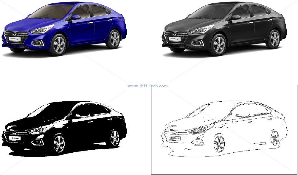
Contours

References:

• Contours: Getting Started, OpenCV Docs.

import numpy as np
import cv2
from matplotlib import pyplot as plt

im = cv2.imread('hyundai-verna.jpg')
imBlank = np.ones(im.shape)
imGray = cv2.cvtColor(im,cv2.COLOR_BGR2GRAY)
imThresh, contours, hierarchy = \
    cv2.findContours(
        cv2.threshold(imGray, 125, 255, 0)[1],
        cv2.RETR_TREE,
        cv2.CHAIN_APPROX_SIMPLE)
cv2.drawContours(imBlank, contours, -1, (0,0,0), 1)

fig, axs = plt.subplots(nrows = 2, ncols=2)
axs[0][0].imshow(im, cmap = 'gray'),       axs[0][0].axis('off')
axs[0][1].imshow(imGray, cmap = 'gray'),   axs[0][1].axis('off')
axs[1][0].imshow(imThresh, cmap = 'gray'), axs[1][0].axis('off')
axs[1][1].imshow(imBlank, cmap = 'gray'),  axs[1][1].axis('off')

fig.show()
plt.show()

Outputs the following: