Notes on some linear algebra topics. Sometimes I find things are just stated
as being obvious, for example, the dot product of two orthogonal vectors
is zero. Well... why is this? The result was a pretty simple but
nonetheless it took a little while to think it through properly.
Hence, these notes... they started of as my musings on the "why", even if the
"why" might be obvious to the rest of the world!
A lot of these notes are now just based on the amazing Khan Academy linear algebra tutorials. In fact, id say the vast majority are... they are literally just notes on Sal's lectures!
A vector is an element of a vector space. A vector space, also known as a
linear space, , is a set which has addition and scalar multiplication defined
for it and satisfies the following for any vectors , , and and scalars
and :
1
Closed under addition:
2
Communative:
3
Associative:
4
Additive identity:
5
Inverse:
6
Closed under scalar multiply:
7
Distributive:
8
Distributive:
9
Distributive:
10
Multiply identity:
Functions Spaces
First let's properly define a function. If and are sets and we have and ,
we can form a set that consists of ordered pairs . If it is the case that
, then is a function and
we write . This is called being "single valued", i.e., each input to the
function is unambiguous. Note, is not a function, it is the value returned by
the function: is the function that defines the mapping from elements in (the domain)
to the elements in (the range).
One example of a vector space is the set of real-valued functions of a real variable, defined
on the domain . I.e., we're talking about where
each is a function. In other words, with the
aforementioned restriction on the domain.
We've said that a vector is any element in a vector space, but usually we thing of this in
terms of, say, . We can also however, given the above, think of functions
as vectors: the function-as-a-vector being the "vector" of ordered pairs that make
up the mapping between domain and range. So in this case the set of function is still like a
set of vectors and with scalar multiplication and vector addition defined appropriately the
rules for a vector space still hold!
What Isn't A Vector Space
It sounded a lot like everything was a vector space to me! So I did a quick bit of googling
and found the paper
"Things that are/aren't vector spaces".
It does a really good example of showing how in maths we might build up a model of something and expect it
to behave "normally" (i.e., obeys the vector space axioms), but in fact doesn't, in which
case it becomes a lot harder to reason about them. This is why vectors spaces are nice... we can
reason about them using logic and operations we are very familiar with and feel intuitive.
Linear Combinations
A linear combination of vectors is one that only uses the addition and scalar multiplication
of those variables. So, given two vectors, and the following are linear
combinations:
This can be generalise to say that for any set of vectors
that a linear combination of those vectors is .
Spans
The set of all linear combinations of a set of vectors is called the span of those vectors:
The span can also be refered to as the generating set of vectors for a subspace.
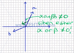
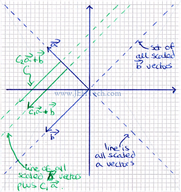
In the graph to the right there are two vectors and . The dotted blue lines show
all the possible scalings of the vectors. The vectors span those lines. The green lines show
two particular scalings of added to all the possible scalings of . One can
use this to imagine that if we added all the possible scalings of to all the possible
scalings of we would reach every coordinate in . Thus, we can say that
the set of vectors spans , or .
From this we may be tempted to say that any set of two, 2d, vectors spans but we
would be wrong. Take for example and . These two variables are
co-linear. Because
they span the same line, no combination of them can ever move off that line. Therefore they
do not span .
Lets write the above out a little more thoroughly...
The span of these vectors is, by our above definition:
Which we can re-write as:
... which we can clearly see is just the set of all scaled vectors of . Plainly,
any co-linear set of 2d vectors will not span .
Linear Independence
We saw above that the set of vectors are co-linear and thus did
not span . The reason for this is that they are linealy dependent, which
means that one or more vectors in the set are just linear combinations of other vectors
in the set.
For example, the set of vectors spans , but is
redundant because we can remove it from the set of vectors and still have a set that spans .
In other words, it adds no new information or directionality to our set.
A set of vectors will be said to be linearly dependent when:
Thus a set of vectors is linearly independent when the following is met:
Sure, this is a definition, but why does this mean that the set is linearly dependent?
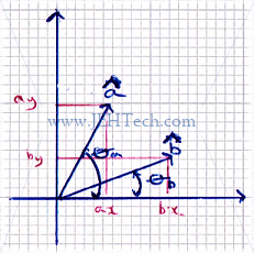
Think of vectors in a . For any two vectors that are not co-linear, there is
no combination of those two vectors that can get you back to the origin unless they are both
scaled by zero. The image to the left is trying to demonstrate that. If we scale , no matter
how small we make that scaling, we cannot find a scaling of that when added to
will get us back to the origin. Thus we cannot find a linear combination where
and/or does not equal zero.
This shows that neither vector is a linear combination of the other, because if it where, we could
use a non-zero scaling of one, added to the other, to get us back to the origin.
We can also show that two vectors are linearly independent when their dot product is zero. This
is covered in a latter section.
Another way of thinking about LI is that there is only one solution to
the equation .
Linear Subspace
If is a set of vectors in , then is a subspace of
if and only if:
contains the zero vector:
is closed under scalar multiplication:
is closed under addition:
What these rules mean is that, using linear operations, you can't do anything to "break" out
of the subspace using vectors from that subspace. Hence "closed".
Surprising, at least for me, was that the zero vector is actually a subspace of because the set
obeys all of the above rules.
A very useful thing is that a span is always a valid subspace. Take, for example,
. We can show that it is a valid subspace by checking that it
objects the above 3 rules.
First, does it contain the zero vector? Recall that a span is the set of all linear combinations
of the span vectors. So we know that the following linear combination is valid, and hence the
span contains the zero vector.
Second, is it closed under scalar multiplication? Because the span is the set of all
linear combinations, for any set of scalars ...
... must also be in the subspace, by definition of a subspace!
Third, is it closed under vector addition? Well, yes, the same argument as made above would
apply.
Interestingly, using the same method as above, we can see that even something trivial,
like the , which is just a line, is a subspace of .
It can also be shown that any subspace basis will have the same number of elements. We say that the dimension of a subspace is the number of
elements in a basis for the subspace. So, for example, if we had a
basis for our subspace consisting of 13 vectors, the dimension of the subspace would be lucky 13.
Basis Of A Subspace
Recall,
is a subspace of (where each vector ). We also
know that a span is the set of all possible linear combinations of these vectors.
If we choose a subset of , , where all the vectors in are linearly independent,
an we can write any vector in as a linear combination of vectors in ,
then we say that is a basis for .
acts as a "minimal" set of vectors required to span . I.e., if you added any
other vector to it is superfluous, because it would be a linear combination of the vectors
already in . You don't add any new information.
Put more formally: Let be a subspace of . A subset is a basis for iff the following are true:
The vectors span , and
They are linearly independent.
A subspace can have an infinite number of basis, but there are standard basis. For
example in the standard basis is . The rule of invariance of dimension states that two bases for a subspace contain the same number of vectors. The number of elements in the basis for a subspace is called the subspace's dimension, denoted as , where is the subspace.
Thus, we can say that every subspace of has a basis and .
A basis is a good thing because we can break down any element in the space that the basis
defines into a linear combination of basic building blocks, i.e. the basis vectors.
To find a basis use the following method:
Form a matrix where the jth column vector is the jth vector .
Reduce the matrix to row-echelon form.
Tak the column vectors that contain a pivot and these are the basis vectors.
TODO discuss the canonical vectors in R2 and R3. , ... but we could also have , .
TODO unique coefficients. implied by the linear independence
TODO most important basis are orthogonal and orthonormal.
Orthonormal are good because we can find the coefficient in the new basis easily:
The dot product is one definition for a vector multiplication that results in a scalar.
Given two equal-length vectors, the dot product looks like this:
Written more succinctly we have:
The dot product is important because it will keep popping up in many places. Some particular
uses are to calculate the length of a vector and to show that two vectors are linearly
independent.
Properties
The operation has the following properties:
Commutative:
Distributive:
Associative
Cauchy-Schwartz Inequality
,
where is non-zero.
Vector Triangle Inequality
Angle Between Vectors
The dot product also defines the angle between vectors. Take two unit vectors and .
We can calculate:
We know that:
And we know that:
Therefore, by substitution:
Thus, describes the angle between unit vectors. If the vectors are not unit
vectors then the angle is defined, in general, by:
Vector Length
Vector Transposes And The Dot Product
In linear algebra vectors are implicitly column vectors. I.e., when we talk about we mean:
Thus, the transpose of is a row vector:
We can then do vector multiplication of the two like so:
So, in general .
Dot Product With Matrix Vector Product
If is an mxn matrix and then .
Then, if then is also well defined and:
Thus we can say .
Unit Length Vectors
A unit vector is a vector that has a length of 1. If is a vector (notice the special symbol used)
then we defined its length as:
Thus if a vector is a unit vector then .
Interesting we can also write .
To construct a unit vector where , we
need the sum to also be 1! How do we achieve this if ? We do the following:
Orthogonal Vectors and Linear Independence
Figure 1
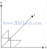
Orthogonal vectors are vectors that are perpendicular to each other.
In a standard 2D or 3D graph, this means that
they are at right angles to each other and we can visualise them
as seen in Figure 1: is at 90 degrees to both and .
is at 90 degrees to and , and is at
90 degrees to and .
In any set of any vectors, , the vectors will be linearly independent if every vector in the set
is orthogonal to every other vector in the set. Note, however that whilst an orthogonal set is L.I., a L.I. set is not necessarily
an orthogonal set. Take the following example:
The vectors and are L.I. because nethier can be represented as a linear combination of the other. They are not
however orthogonal.
So, how do we tell if one vector is orthogonal to another? The answer is
the dot product which is defined as follows.
We know when two vectors are orthogonal when their dot product is
zero: x and y are orthogonal. You can scale either or both vectors and their dot product will still be zero!
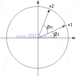
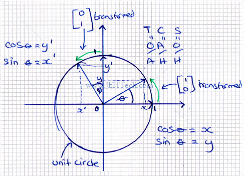
But why is this the case? Lets imagine any two arbitrary vectors, each
on the circumference of a unit circle (so we know that they have the
same length and are therefore a proper rotation of a vector around the
center of the circle). This is shown in figure 2. From the figure, we
know the following:
Figure 2
The vector is the vector rotated by degrees.
We can use the following
trig identities:
Substitute these into the formulas above, we get the following.
Which means that...
For a 90 degree rotation we know that
and . Substiuting these values into the above equations
we can clearly see that...
Therefore, any vector in 2D space that is will become
and therefore the dot product becomes . And
voilà, we know know why the dot product of two orthogonal 2D vectors is
zero. I'm happy to take it on faith that this extrapolates into n dimensions :)
Another way of looking at this is to consider the law of cosines: :
Here and represent the magnitude of the vectors , , and , . represents
the magnitude of the vector . Thus, we have this:
I.e., .
When the angle between the vectors is 90 degrees, and so that part of the
equation disappears to give us .
Now...
Recall that and that therefore .
Based, on this we can say that...
Now, all of the and terms above will be cancelled out by the and terms,
leaving us with...
Which is just twice the dot product when the vectors are at 90 degrees - or just the dot product because we can divide through by 2.
Matrices
Properties
Khan Academy has great articles. This is another good reference from MIT.
Scalar Multiplication
Associative:
Distributive: and
Identity:
Zero:
Closure: is a matrix of the same dimensions as .
Note that scalar multiplication is not commutative: !
Matrix Addition
Commutative:
Associative:
Zero: For any matrix , there is a unique matrix such that
Inverse:
Closure: , is a matrix of the same dimensions as and .
Matrix Multiplication
Associative:
Distributive:
Identity:
Zero:
Inverse: Only if is a square matrix, then is its inverse and . Note that not all matrices are invertible.
Dimension: If is an matrix and is an matrix then is an matrix.
Note that matrix multiplication is not commutative: !
Be careful: the equation does not necessarily mean that or and for
a general matrix , , unless is invertible.
Matrix Transpose
Associative:
Distributive (into addition):
Distributive (into mult):
Generalises to
Identity:
Inverse:
Name?:
Name?:
Name?:
If columns of are LI then columns of are LI. is square and also invertible.
Matrix Inverse
Associative (self with inverse):
Distributive (into scalar mult):
Distributive (into mult):
Identity:
Name?:
Name?:
Matricies, Simultaneous Linear Equations And Reduced Row Echelon Form
The set of linear equations:
Can be represented in matrix form:
Any vector , where , is a solution to the set of simultaneous
linear equations. How can we solve this from the matrix. We create an augmented or patitioned matrix:
Next this matrix must be converted to row echelon form. This is where each row has
the same or less zeros to the left than the row below. For example, the following matrix is
in row echelon form:
But, this next one is not:
We go from a matrix to the equivalent in row-echelon form using elementary row operations:
Row interchange:
Row scaling:
Row addition:
In row echelon form:
All rows containing only zeros appear below rows with nonzero entries, and
The first nonzero entry in any row appears in a column to the right of the first nonzero entry in any preceding row.
The first non zero entry in a row is called the pivot for that row.
And woop, woop, even more important than echelon form is reduced row-echelon form (rref). This is when:
If a row has all zeros then it is below all rows with a non-zero entry.
The left most entry in each row is 1 - it is called the pivot.
The left most non-zero entry in each row is the only non-zero in that column.
Each row has more zeros to the left of the pivot than the row above.
Or, to put it another way, when it is a matrix in row-echelon form where:
All pivots are equal to 1, and
Each pivot is the only non-zero in its column.
Some important terms are pivot position and pivot column. The position is the location of a leading 1, which meets the above criteria, and the column is a column that contains a pivot position.
So why do we give a damn above RREF if we have row-echelon form? Well, one reason is it lets us
figure out if a set of linear equations has a solution and which variables are free and
which are dependent. The reason for this is that the RREF of every matrix is unique (whereas merely row reducing a matrix can have many resulting forms).
The free variable is one that you have control over, i.e. you can choose and manipulate its value.
The dependent one depends on the values of the other variables in the experiment or is constant.
Pivot columns represent variables that are dependent. Why?
Recall that the column vector containing a pivot is all-zeros except
for the pivot. So if element j in a row of a rref matrix is a pivot, then in our
system of equations only
appears in this one equations in our RREF matrix. Thus, its value must be determined as this is
the only place it occurs. It must either be a constant or a combination of other variables.
Because column vectors containing a pivot are all-zeros except
for the pivot, the set of pivot columns must also be LI (see later).
You can always represent the free columns as linear combinations of the
pivot columns.
If we have an augmented matrix :
No Solution. If the last (augmented) column of (ie. the column which contains
) contains a pivot entry.
Restructed Solution Set. If the last row of the matrix is all zeros except the pivot column which is a function of .
Exactly One Solution. If the last (augmented) column of (ie. the column which contains
) does not contain a pivot entry and all of the columns of the coefficient part (ie. the columns
of ) do contain a pivot entry.
Infinitely Many Solutions. If the last (augmented) column of (ie. the column which contains
) does not contain a pivot entry and at least one of the columns of the coefficient part
(ie. the columns of ) also does not contain a pivot entry.
Let's look at a quick example of a matrix in echelon-form:
We can get the solution to the set of simultaneous linear equations using back substitution. Directly
from the above row-echelon form (useful because the last row has one pivot and no free variables) matrix we know that:
From (1) we know:
Substitute (4) back into (2):
Substitute (5) and (4) back into (1):
We can use RREF to accomplish the same thing and find the solutions to the above.
Which means we come to the same conclusion as we did when doing back substitution, but were able to
do it using elementary row operations.
We can not talk about the general solution vector, , which in this case is:
We can also talk about the solution set, which is the set of all vectors that result in a valid solution to our system of equations. In this case our solution set is trivial: it just has the above vector in it because the RREF had pivots in every column so there is exactly one solution.
Lets, therefore, look at something more interesting. Take the RREF matrix below:
Now we have two free variables! Now and where and can be any values we like. Now the general solution vector looks like this:
How did we get here? We we know from the RREF matrix that:
We replace and with our free variables and then solve for the pivots, thus getting the general solution vector.
The above can then be represented using the general solution vector:
The solution set thus becomes:
We can find the reduced row echelon form of a matrix in python using the sympy package and the rref() function:
from sympy import Matrix, init_printing

init_printing(use_unicode=True)

system = Matrix(( (3, 6, -2, 11), (1, 2, 1, 32), (1, -1, 1, 1) ))
system
system.rref()[0]
Which outputs:
⎡1  0  0  -17/3⎤
⎢              ⎥
⎢0  1  0  31/3 ⎥
⎢              ⎥
⎣0  0  1   17  ⎦
To then apply this to our augmented matrix we could do something like the following. Lets
say we have a set of 3 simultaneous equations with 3 unknowns:
We'd make an augmented matrix like so:
To solve this using Python we do:
from sympy import Matrix, solve_linear_system, init_printing
from sympy.abc import x, y, z

init_printing(use_unicode=True)

system = Matrix(( (3, 6, -2, 11), (1, 2, 1, 32), (1, -1, 1, 1) ))
system

solve_linear_system(system, x, y, z)
Matrix/vector multiplication is pretty straight forward:
The concept of matrix multiplication, the type I learnt in school, is
shown in the little animation below. For each row vector of the LHS matrix
we take the dot product
of that vector with each column vector from the RHS matrix to produce the result:
But having said that, I'd never really thought of it as shown below until watching some
stuff on Khan Academy:
We can think of it as the linear combination of the column vectors of the matrix where
the coefficients are the members of the vector, where the first column vector is multiplied
by the first element, the second column vector by the second element and so on.
So, for any mxn matrix, , and vector we can say that,
Null Space Of A Matrix
Definition
For an nxm vector , the nullspace of the nxm matrix , is defined as follows:
In words, the null space of a matrix is the set of all solutions
that result in the zero vector, i.e. the solution set to the above. We can get this set by using the normal reduction to RREF to solve the above (). The solution space set to this is the null space.
The system of linear equations is called homogeneous. It is always
consistent, i.e., has a solution, because is always a solution (and is called the trivial solution).
The null space of a matrix is a valid subspace of because
it satisfies the following conditions, as we saw in the
section on subspaces.
The nullspace of a matrix can be related to the linear independence of it's column
vectors. Using the above definition of nullspace, we can write:
Recalling how we can write out vector/scalar multipication,
we get,
Recall from the section on linear independence that the above set of vectors
is said to be linearly dependent when:
Given that our nullspace is the set of all vectors that satisfy the above, by definition,
then we can say that the column vectors of a matrix A are LI if and only if .
Relation To Determinant
If the determinant of a matrix is zero then the null space will be non trivial.
Calculating The Null Space
To find the null space of a matrix , augment it with the zero vector and convert it to RREF. Then the solution set is the null space. So,
if there are only pivots, the null space only contains the zero vector because there is only one solution (which therefore must be 0).
Example #1
Let's look at a trivial example:
Then the null space is defined as the solution set to , i.e...
We find the solution set using the normal augmented matrix method:
There are no free variables, so therefore the solution set can contain only the zero vector because we have three contraints and . The only values for the 's that can satisfy these constrains is zero, hence the null space can only contain the zero vector.
Example #2
Lets try an consider another trivial example.
It's pretty contrived because I constructed it by applying row operations to the identify matrix! Null space is defined as solutions to:
We find the solution set using the normal augmented matrix method:
Now we can see that and . The variable , however, is free. It can take any value. Let's call that value . The solution vector is therefore:
The general solution vectors is therefore:
So we can say the null space is:
Example #3
Let's try one more example. This one is right out of Khan Achademy rather then my own made up rubbish :)
We calculate the null space by setting up an augmented matrix to solve for :
We thus know that:
And that and are free variables. This means that the general solution is:
And therefore we can define the null space as:
An Intuitive Meaning
This StackOverflow thread gives some really good intuitive meaning to the null space. I've quoted some of the answers verbatim here:
It's good to think of the matrix as a linear transformation; if you let , then the null-space is ... the set of all vectors that are sent to the zero vector by . Think of this as the set of vectors thatlose their identity as is applied to them.
Let's suppose that the matrix A represents a physical system. As an example, let's assume our system is a rocket, and A is a matrix representing the directions we can go based on our thrusters. So what do the null space and the column space represent?
Well let's suppose we have a direction that we're interested in. Is it in our column space? If so, then we can move in that direction. The column space is the set of directions that we can achieve based on our thrusters. Let's suppose that we have three thrusters equally spaced around our rocket. If they're all perfectly functional then we can move in any direction. In this case our column space is the entire range. But what happens when a thruster breaks? Now we've only got two thrusters. Our linear system will have changed (the matrix A will be different), and our column space will be reduced.
What's the null space? The null space are the set of thruster intructions that completely waste fuel. They're the set of instructions where our thrusters will thrust, but the direction will not be changed at all.
Another example: Perhaps A can represent a rate of return on investments. The range are all the rates of return that are achievable. The null space are all the investments that can be made that wouldn't change the rate of return at all.
Nullity Of A Matrix
The dimension of a subspace is the number of elements in a basis for that subspace. The dimension of
the null space is called the "nullity":
In the null space you will always have as many vectors as you have free variables in the RREF of the matrix. So the nullity is the number of free variables in the RREF of the matrix with which this null space is associated:
This the null space has dimension, or nullity, . This equates to the number of free variables.
Column Space Of A Matrix
The columns space of a matrix is the set of all linear combinations
of its column vectors, which is the span of the column vectors:
Note that the column vectors of might not be LI. The set can be
reduced so that only the LI vectors are used, which means the above still holds,
and then we say that the LI set is a basis for .
The column space of A is a valid subspace.
For the system of equations , is the set of all values that can be. We can look at this this way:
The solution, , can be seen to be a linear combination of the column vectors of . Thus, .
Therefore, if and ,
then we know that no solution exists, a conversely, if it is then we know
that at least one solution exists.
The set of vectors in the column space of may or may not be linearly independent. When reduced to being LI then we have a basis for the
column space of the matrix.
We saw the following in the section of null spaces: It can be shown that the column vectors of a matrix are LI if and only if . So we can figure out if we have a basis by looking at 's
null space. Recall that and
that the column vectors of a matrix A are LI if and only if !
How do we figure out the set of column vectors that are LI? To do this,
put the matrix in RREF and select the columns that have pivot entries (the pivot columns).
The pivot column vectors are the basis vectors for :) The reason is that you can always write the columns with the free variables
as linear combinations of the pivot columns.
Because column vectors containing a pivot are all-zeros except
for the pivot, the set of pivot columns must also be LI.
You can always represent the free columns as linear combinations of the
pivot columns.
So to find column space of , pick the columns from that correspond
to (have the same position as) the pivot columns in .
A really interested property of the column space is the column space criterion which states that a linear system, has a solution iff is in the column space of A.
Rank Of A Matrix
We can now define what the rank of a matrix is:
I.e., The rank of a matrix is the number of pivots. This also means that the rank is the number of vectors in a basis for the column space of .
You can get this by counting the pivot columns in .
The rank equation is , where is an matrix.
If is reduced to row-echelon form , then:
is the number of free variables in solution space of , which equals the number of pivot-free columns in .
... a "basis of a column space" is different than a "basis of the null space", for the same matrix....
A basis is a a set of vectors related to a particular mathematical "space" (specifically, to what is known as a vector space). A basis must:
be linearly independent and
span the space.
The "space" could be, for example: , , , ... , the column space of a matrix, the null space of a matrix, a subspace of any of these, and so on...
Orthogonal Matrices
So, onto orthogonal matrices. A matrix is orthogonal if .
If we take a general matrix and multiply it by it's transpose we get...
The pattern looks pretty familiar right?! It looks a lot like
, our formula for the dot product of two vectors. So,
when we say , , and , we will get the following:
a matrix of two row vectors, .
If our vectors and are orthogonal,
then the component must be zero. This would give us the first
part of the identify matrix pattern we're looking for.
The other part of the identity matrix would imply that we would have
to have and ... which are just the
formulas for the square of the length of a vector.
Therefore, if our two vectors are normal (i.e, have a length of 1), we
have our identity matrix.
Does the same hold true for ? It doesn't if we use our original
matrix A!...
Oops, we can see that we didn't get the identity matrix!! But, perhaps we
can see why. If was a matrix of row vectors then is a matrix
of column vectors. So for we were multiplying a matrix of row vectors
with a matrix of column vectors, which would, in part, give us the dot
products as we saw. So if we want to do it would follow that for
this to work now was to be a matrix of column vectors because
we get back to our original ( would become a mtrix of row vectors):
So we can say that if we have matrix who's rows are orthogonal vectors
and who's columns are also orthogonal vectors, then we have
an orthogonal matrix!
Okay, thats great n' all, but why should we care? Why Are orthogonal
matricies useful?. It turns our that orthogonal matricies
preserve
angles and lengths of vectors. This can be useful in graphics to rotate
vectors but keep the shape they construct, or in numerical analysis
because they do not amplify errors.
Determinants
The Fundamentals
If is defined as follows...
Then we write the determinate of B as...
A matrix is invertible iff . We can define the inverse as follows using the determinant:
It is defined as long as .
If is a 3x3 matrix defined as follows, where the elements represents the element at row and column :
We can define the determinant as:
Same rule applies: If the determinant is not zero then the matrix will be invertible.
We've used the first row () but we could have used any row, or any column: choose
the one with the most zeros as this will make the calculation easier/faster.
Select the row or column with the most zeros and go through it. Use each element multiplied by the determinant of the 2x2 matrix you get if you take out the ith row and jth column of
the matrix.
This generalises to an nxn matrix as follows:
Define to be the (n-1) x (n-1) matrix you get when you ignore the ith and jth column of the nxn matrix A.
Then we can define the determinant recursively as follows:
For each , apply the formula recursively until a 2x2 matrix is reached, at which point you
can use the 2x2 determinant formula.
There is a pattern to the "+"'s and "-"'s:
A quick example. is defined as follows:
We find the determinant as follows, where as we did previously, we define to be the (n-1) x (n-1) matrix you get when you ignore the ith and jth column of the nxn matrix A.
See how the 4th row was used as it contains 2 zeros, meaning that we only have to actually do
any work for two of the terms. Note also how we got the signes for the various components using . Another way to visualise this is shown below:
This now needs to be applied recusively, so we figure out the determinants of and in the same way.
Let :
Note again how we picked row 2 because it only had 1 term which was non-zero and hence made our life easier.
Let
We picked row 2 again, but we could have just as easily used columns 1 or 3 to the same effect.
Now we can write:
We can see this answer verified in the section "Do It In Python"
The following is an online matrix determinant calculator app, written in Javascript, to explain calculation of determinant. Define a matrix in the text box
using a Matlab-like sytax. For example, "1 2 3; 3 4 5; 5 6 7", defines the 3x3 matrix:
Use it to create matricies to see, step by step, with explanations, how the determinant is calculated. Just replace the text in the message box below and hit the button to see how you can solve for the determinant of your matrix...
Rule Of Sarrus
For a 3x3 matrix defined as follows:
The determinant is defined as:
Notice how it is the diagonals (wrapped) summed going from left to right, and the diagonals (wrapped) subtracted going from right to left.
Effect When Row Multiplied By Scalar
Multiplying a row in a matrix by a scalar multiplies the determinant by that scalar. This is shown anecodtally below.
Effect When Matrix Multiplied By Scalar
Multiplying an entire nxn matrix by a scalar, scales the determinant by n2. Shown anecdotally below:
Row Op: Effect Of Adding A Multiple Of One Row To Another
Say that A is defined as follows:
Now lets say we apply the row operation Row1 = R1 + kR2 to get the matrix:
Now...
I.e. adding a multiple of one row to another doesn not change the determinant, as shown
anecdotally above! Works that same if we do Row1 = R1- kR2.
Row Op: Effect Of Swapping Rows
Swapping A's rows and taking the determinant gives us:
So, we can see that for a 2x2 matrix, swapping rows changes the sign of the determinant. Generalise to nxn.
Effect Of Adding A Row From One Matrix To Another
Let's say we have two matricies:
Create a new matrix by adding the second column of A to B:
We will find out that the derminant of Z is the sum of the determinants for A and B:
Generalises to nxn matricies.
When A Matrix Has Duplicate Rows
We have seen that when we swap two rows that the determinant is negated. But, if we swap two
identical rows the matrix determinant should not change! The only way this can be true is if
the determinant is zero.
This, somewhat anecodtally, we can say that if a matrix has a duplicate row then it's determinant
must be zero! The same is true if one row is a simple scalar multiple of another.
We have also seen that the inverse of a matrix is only available when its determinant is
non-zero. Therefore we now know that matricies with duplicate rows are not invertible.
Same still applies if on row is a scalar multiple of another.
Upper Triangular Determinant
An upper triangular matrix is one where everything below the diagonal is zero. For upper
triangular matricies the determinant is the multiplication of the diagonal terms:
And:
This generalises to nxn matricies:
The same applies to lower triangular matrixies.
This method gives us a way of getting more efficient determinants for matricies if we can get them into an upper or lower diagonalisation. The Khan lectures give this example of a matrix reduction (remember that we saw that adding multiples of one row to another does not change the determinant):
Note the minus because a row was swapped to do the reduction!
The Determinant And The Area Of A Parallelogram
This is one of the better YouTube tutorials I've found that explains the concepts and not just the
mechanics behind determinants, by 3BlueBrown (awesome!).
Now, onto more notes from Khan Academy, which also give an abolsolutely awesome explanation! Also, this Mathematics StackExchange Post gives
loads of different ways of proving this.
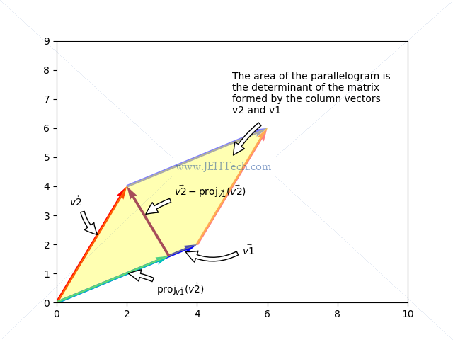
For two vectors, each made a column vector of a matrix A, the determinant of A gives the area of the parallelogram formed by the two vectors:
Put a little more mathsy-like, if you have two vectors, call them, and , then
the area of the parallelogram formed by the vectors, as shown above, is given by:
To aid in the following explanation you might need to refer to the section on projections.
The area of a parallelogram is given by the base times the height. In the above we can see that the base
of the parallelogram is just the length . The height of the parallelogram, we can
see is . So...
Get rid of the square roots by squaring both sizes:
Now we have to solve the dot products, which means we will have to define our two vectors like so:
Substituting these vector definitions into the above we can expand out the dot products:
Now, in the section on linear transforms, we will see that the columns vectors of the transform matrix show what happens to the canocial basis vectors. Thus, if the determinant of the transformation matrix is the area of the parallelogram formed by the column vectors of the matrix, the determinant gives us the scaling factor of the transformation!
Rowspace & Left Nullspace & Orthogonal Complements
We saw in the 3rd null space example the following matrix, and its reduction to RREF:
We calculate the null space by setting up an augmented matrix to solve for :
Giving...
But, we also know that because only the first column in the RREF form has a pivot entry, the basis for the column space of the matrix only contains the first column vector:
We also know the rank of the matrix:
Now we take the transpose of :
So, now we can calculate the nullspace of the transpose of A. We see that and that is a free variable so:
The is called the left null space of . Why have we called in the left null space?
Have a look at this...
...by the very definition of what a null space is. We are solving for :
Thus, the null space of can also be defined as so:
Now we see why it is called the "left" null space: the vector is on the LHS of the transformation matrix!
Rowspace
The rowspace of the transformation is defined as :
Recall from above:
The only pivot column is the first, so:
Relationship Between The Spaces: Orthogonal Complements
An orthogonal complement is defined as follows. If is a subspace of , the orthogonal complement of is written as is defined as so:
In other words, every member of is orthogonal to every member of .
It can be shown that is a valid subspace: it is closed under addition and scalar multiplication.
To find the orthogonal complement of , take its generating vectors and place them as row vectors in a matrix. If, and the generating set of vectors, or span, of is then form the by matrix:
In the above matrix, becomes the row space of . Because the null space of is the orthogonal complement of this matrix, the orthogonal compement to your subspace is found by finding the null space of the above matrix!
The null space and row space are perpendicular. They are orthogonal complements. Thus we can say:
We can show that . We want to show that if then for all . We know
that which we can write as:
Where is the ith row vector of .
We know that, by the definition of matrix definition we can say the following:
The above is just the the matrix multiplication shown above written out. But, we know that
is the same as the dot product, so it is equal to . I.e., the row vectors of must all be orthogonal to if is a member of the null space.
Thus, the vectors in the null space are to the column vectors of . Thus,
.
If we let , then and thus .
Relating The Dimension Of A Subspace To Its Orthogonal Complement
The dimensions of each subspace can also be related: , where is a subspace of . This, therefore, means that if , then .
Representing A Vector As A Combination Of A Vector In A Subspace And One In Its Orthogonal Complement
This relation implies that . So, if is a basis for then is a basis for . This
leads us to an importan property where we can say that any vector in can be represented uniquely by some vector in a subspace of and some vector in :
We can also notice something important about the intersection of a subset and its orthogonal complement: if and then . I.e. .
Unique Rowspace Solution To
We have seen that any vector in can be represented as a combination of and .
So if is a solution to , where , then we can express
as where and .
I.e., the solution is a linear combination of some vector in the rowspace of and some vector in the null space of .
Thus, , which means that is a solution!
We have also seen, in the section on the column space that the solution, if it exists, must be in the column space of . Therefore, for any vector, , in the column space of , there is a unique vector, in the rowspace of that is the solution. Woah!!
It can also be shown that this is a unique solution. Proof ommited.
To summarise: any solution to can we written as and we know there is a unique solution in the rowspace of A, .
This means that we can also write:
This is a very important point, as we'll see later on when this gets applied to things like least square
estimation. If , then such that is a solution to and no other solution has a length less than .
Summary
The orthogonal complement of a subspace has the following properties:
is a subspace of .
.
.
Each vector in can be expressed unqiuely in the form for and .
If , then such that is a solution to and no other solution has a length less than
A Visual Exploration
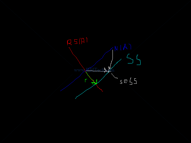
We know that the nullspace of is defined as and that , so we can determine the null space by reducing to its RREF as so:
Now the rowspace, aka :
We have seen that the column space of a matrix will be the column vectors associated with the pivot columns. Therefore:
So, what about the solution set?
We can see that the solution set is a scaled vector from the null space plus some particular solution. These can be plotted as so:
We can also see that, as we discovered previously, the shortest solution to the problem is the vector
formed by the null-space vector scaled to zero plus a vector in the rowspace:
Eigenvectors and values exist in pairs: every eigenvector has a corresponding eigenvalue. An eigenvector is a direction, ... An eigenvalue is a number, telling you how much variance there is in the data in that direction ...
Linear Transformations
Functions
Scalar Functions
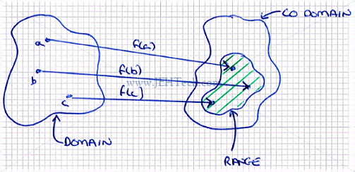
Normally a function is a mapping between two sets: from a domain to a range, which is
a subset of the function's co-domain. I.e., the co-domain is the set of all possible things the
function could map onto and the range is the subset of the co-domain containing the things the
function actually maps to. If we have two sets, and , we say that if is a function, then it associates elements of with elements of . I.e., is a mapping between and , and we write .
The usual function notation looks like this: . Note that is the function,
not , which is the value output by the function, , when is input. There are
other notations we use to denote functions.
For example the function can be described as a mapping from the
set of all real numbers to the set of all real numbers.
It can also be defined using this notation:
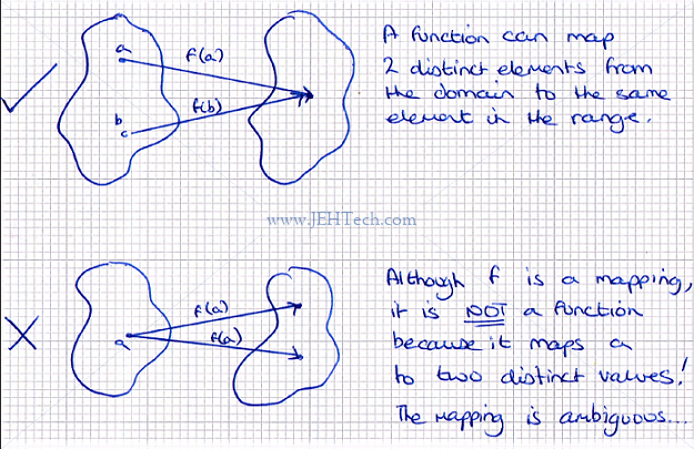
A function is not, however, a simple mapping between two sets. For a mapping to be a function
the following must be true: . In other words
one item in the domain cannot map to more than one item in the range, but two distinct
items in the domain can map to the same item in the range.
Vector Valued Functions
Functions that map to are called scalar values functions, or specifically in
this case, real valued functions.
If the co-domain of a function is in , where , then we say that the function
is vector valued. Functions, where the domain is in are called
transformations.
A vector values function could like something like this, for example:
It could look like anything... the point is, because operates on a vector, we
call it a transformation.
Surjective (Onto) Functions
A surjective, or onto, function provides a mapping from the domain to
every element of the co-domain. I.e., the range is the
co-domain, or the image of the function is the co-domain. If and is surjective, then .
TODO: Insert diagram
Injective (One-To-One) Functions
An injective, or one-to-one, function provides a mapping to every element
of the co-domain such that no two elements from the domain can map to the
same value in the co-domain. Note that not all domain members need to be
mapped however.
TODO: Insert diagram
Bijective (One-To-One And Onto)
A function is bijective (one-to-one and onto) when it is both surjective (onto) and injective (one-to-one).
TODO: Insert diagram
Invertible Functions
A function is invertible if there exists another function such that .
In the above is the identity function: where .
If a function is invertible then the function is unique and there is only one unique
solution to .
To summarise, the function is invertible iff,
Which means that there is only one solution to , so we
can also say:
The part of the expression, implies that the range of the function is the co-domain, which means that the function is surjective (onto) and the part of the expression means that the function is also injective (onto), which thus means that the function is bijective (one-to-one and onto).
Thus to be invertible a function must be bijective (one-to-one and onto)!!
Linear Transformations
Vector valued functions are transformations. Linear transformations are a particular
type of transformation that obey the following rules. If and
then:
In other words, the origin must remain fixed and all lines must remain lines. For example, a transformation such as is non linear because , generally, for example.
Matrices are used to do the linear transformations so the function will generally
be defined as , where is the transformation matrix. 2D
vectors transform 2D space, 3D vectors transform 3D space and so on...
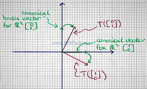
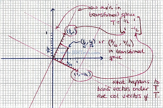
Interestingly the column vectors of the transformation vector , tell us what
happens to the canonical basis vectors in that space, and from this we can work out
how any vector would be transformed.
We have seen that in cartesian space, , for any coordinate, , the
numbers and are the coefficients of the canonical basis vectors...
Lets say our transformation matrix has the following properties:
Well, we've seen we can re-write any vector as a combination of the above basis vectors, so
we can write:
Which looks suspiciously like a matrix, vector product. If we describe the transformation, as follows:
Then...
An so we can see that the first column vector of shows us where the first canonical basis vector maps to
and the second column vector of shows us where the second canonical basis vector maps to... woop!
In other words, just to be clear...
We can also note that this the same as taking the transform of each of the column vectors of the identity matrix!
We can see this more "solidly" in the sketch below...
We can see how one coordinate can be represented using the canonical Cartesian coordinates, but also coordinates in
our transformed space. Thus the same "point" can be represented using different coordinates
(coefficients of the basis vectors) for different transform spaces.
Another important point is that it can be shown that all matrix-vector products are linear transformations!
Linear transformations also have these important properties, if we take two transformations
and , where
has the transformation matrix and has the transformation matrix :
Transformation addition: .
Scalar multiplication: .
Inverse Linear Transformations
We saw in the section on functions that an invertible function has to be
bijective (one-to-one and onto). As a transform is just a vector valued
function, the same condition for invertibility exists. Recall that:
Where the red inidcates that the range is the domain (mapping is surjective or onto) and the blue
indicates that the mapping is unqiue (injective or onto-to-one). We can also write this as follows:
It can be shown that invertibility implies a unique solution to .
We want to understand under what conditions our standard linear transform,
, is invertible.
i.e. when is it both injective (ont-to-one) and surjective (onto)?
Surjective (Onto)
Start with surjective (onto)... we are looking at ,
i.e., ...
We can write as its column vectors multiplied by the elements of :
Remember that a surjective, or onto, function provides a mapping from the domain to every
element of the co-domain. Thus for our transform to be surjective (onto) the set of the above
linear combinations must span .
This means that for to be sujective (onto) the column vectors of have to span
, i.e., the column space of must span (look at the equation above to see why). I.e. . Thus, the
challenge becomes finding this out, because if it is true we are half way there to showing
that the transform is invertible.
For the column space to span (i.e. ) we would
need the solution to to have infinitely many solutions. We saw in the
section of RREF that when an augmented matrix is
reduced to RREF we can determine the number of solutions by looking at where the pivots
are.
To recap, when a matrix is in RREF:
Free variables mean many solutions, , which is what we want!
No free variables (all columns have a pivot) means a unique solution, .
Pivot or function in the augmented column means no solution or restricted solution set respectively and .
Thus, to show that a transform is surjective (onto) we need the RREF of the transformation matrix to have at at least one solution... i.e., there is a unique solution or many solutions - the first two items on the list above.
Thus, there must be a pivot in every row of ou matrix , so for be onto we can say .
Injective (One-To-One)
For invertivility, onto is not enough. We need one-to-one as well! It can be shown that the
solution set to is a the set of shifted versions of the null space. I.e.,
assuming that has a solution, the solution set is [Ref].
This means that for to be one-to-one we require the null space of contain only the zero vector. I.e., for a transformation matrix to be one-to-one, its null space must be trivial.
If the null space of is trivial then . Because the column vectors a LI, they form a basis of vectors so .
Thus, the transform is one-to-one if and only if .
Invertible: Injective (One-To-One) and Surjective (Onto)
We saw that to be surjective, , and to be injective, .
Therefore, to be invertible, must be a square matrix. As it's rank is , this also means that every column must contain a pivot, and because all the columns form a basis, i.e., are LI, if we reduce to RREF, it must be the elementary matrix, . Thus, must also be true.
The inverse mapping is also linear. To recap, linearity implies:
and
Finding The Inverse
To find the inverse of a matrix we augment it with the equivalently size elementry matrix and reduce it to RREF.
Let...
Augment with to form and reduce:
Thus,
And we see that it is indeed the inverse because:
And:
As we've seen, if isn't square then don't bother - it doesn't have an inverse. If it is square
and doesn't reduce to RREF, then it is singular and does not have an inverse.
Projections
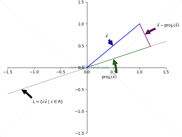
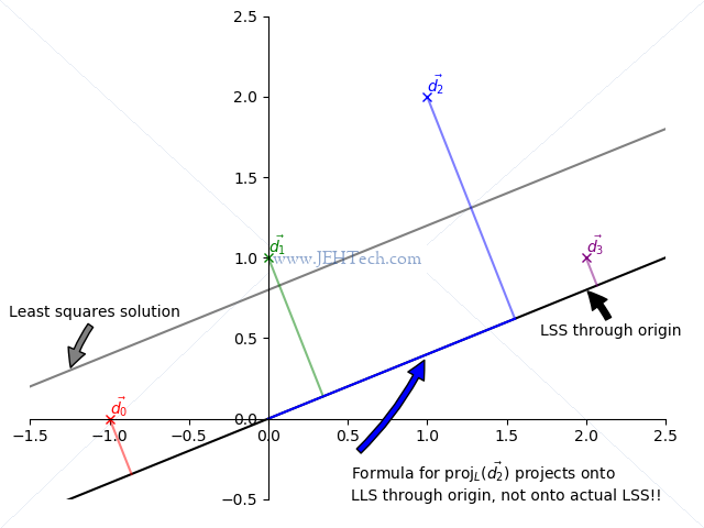
The graph to the below shows a vector and its projection onto the line , defined by the vector .
The projection of onto describes how much of goes in the direction of .
We write "the projection of onto like so:
The projection is found by dropping a line, perpendicular to from the top of , down to . Where this line
hits is the end of the vector that describes the projection. This is shown on the graph by the
smaller green vector labelled , and the purple line labelled .
Because is perpendicular to we can say the following (recall perpendicular vector's dot product is zero):
Thus the projection is defined as:
And if is a unit vector , then this simplifies to:
And we have seen in a previous section how to make a vector a unit vector. Whoopdi do!
An important point to note - which wasn't immediately obvious to me, but probably should've been in hindsight - is that with this projection-onto-a-line, the line projected onto has to pass through the origin! This is seen in better detail later in the second least squares example.
However, I realised this is fine because when we're talking about subspaces they must contain the zero vector, because they are closed under scalar multiplication, so when projecting onto a subspace, the line, plane, or whatever, must pass through the origin! It is only when one starts thinking about graphs or graphics that we need to consider the case where the line doesn't pass through the origin, so this is a case that does not bother us here :)
To calculate the matrix that describes the projection transform,
apply the projection to each of the column vectors of the identity matrix where the column vectors of are the same
length as the vector over which the projection is applied. So, for example, vectors in to get the transformation
matrix for a projection onto a line defined by the vector :
This definition has been defined only for a projection onto a line, which is a valid subspace (recall: closed under addition and scalar multiplication). But what about projections onto planes in 3D or onto any abitrary "space" in ? It does, in fact, generalise to a projection onto any subspace!
If is a subspace of , then we have seen that is also a valid subspace of . We have also seen that we can express any vector in as the sum of a vector in and a vector in .
I.e., if , and , then we can express uniquely as , as we have seen in a previous section. Thus we can say:
Therefore:
And:
We know that a projection is a linear transformation and is therefore defined by some , where is the vector we are projecting, and is the projection of that vector. But, projected onto what? We can see this in the diagram below, which replicates the previous problem's matrix :
We have projected onto the row space of our projection matrix , and the projection is the unique solution from the rowspace. So the row space is, in 2D world, the line we have projected onto, and in any-D world, the subspace we have projected onto. We can say:
In the above problem, the easiest solution was the vector , so we have:
So, we can see the definition of projection for onto a line generalises to a projection onto any subspace
What I'm not clear on so far...

We know how to find the projection matrix for our vector onto a subspace by applying the formula to the column vectors of the identity matrix. So we can get our projection matrix.

Above we've said that the projection is the vector from one of the the othog complements, say V. So the project of an arbitrary vector x onto V will be r if V is the rowspace of the transformation matrix.

So the rowspace of the projection matrix, that we know how to find, must therefore contain r.

To find a projection of x onto V
1. Find the basis vector set for V
2. Find the basis vector set for V^\perp
3. Find the coordinate vector of x relative to the basis vectors of V \union V^\perp - as we can express any vector like this
4. Then b onto V is just the combo of the vector basis components of V

So this must relate projection to change of basis too!! Aaaarg... brain melty
A Projection Onto A Subspace Is A Linear Transform
Say that is a subspace of and that has basis vectors . This means that
any vector can be defined as:
We know from the definition of matrix multiplcation that we can re-write the above as:
Where
Therefore, , we can say for some .
If we have some vector, , then by the definition of a projection. Because,
as we have shown above, , we can say:
We also know that we can say:
Because , by definition of a projection, we must therefore be able to say, because of the equality above that:
Now we note that our matrix, , has the its column vectors set as the basis vectors of . Therefore . We can take the
orthogonal complement of both sides to get . From here, we can recall that
, and that therefore . Armed with this knowlege, we can substitue this into the above to get:
By the definition of a null space, we can say that:
And, we say a couple of stages back that , so we can substitue this in to get:
Now, if was invertible then we can solve for . It was state (without any proof) in the matrix transpose rules list that this is need the case because the columns of , in this case, are LI. Thus:
Because we set , we have found an interesting formula for the projection of onto :
This is a linear transform because is just another matrix! So if we have the basis vectors for our subspace we have a formula to project any vector onto it :)
A Projection Is The Closest Vector In The Subspace Projected Onto
We kinda already saw this. The vector was the shortest solution and this was the projection onto the subspace.
Also the distance from to is the shorter than the distance from to any other vector in :
Least Squares
Lets say we have an by matrix such that:
Lets also say that there is NO solution to the above. We know that we can write out as
. The fact that there is no solution means that there are no coefficients that can satisfy the equation. I.e. .
What we'd like to do is find a vector , which is called our least squares estimate, where is as close as possible to ! I.e., we want to minimise. So whilst may have no solution, is a solution, and it will be the solution with the least error, or distance, from .
Let . Then we are going to minimise . Because is a solution, it means that . So the question is, what vector in 's column space should we pick? Well, we have seen that the projection of a vector onto a subspace is the closest vector in that subspace to the projectee. So we pick the projection of onto the column space of A!
TODO INSERT DIAGRAM TO SHOW THIS
So we want the following, as we know it will produce the least distance between and :
We have previously seen that there is a formula for the projection matrix. We could just use that, but
as Sal continues to explain there is an eaier way - calculating the projection matrix involves a bit of work so lets be lazy :)
Start by subtracting from both sides of the above equation...
Here is orthogonal to .
TDO INSERT DIAGRAM
Thus,
is equal to somthing that is orthogonal to the projection, i.e., . We have also seen
that , so we can re-write the above as:
And, by definition of a null space, will be the set of solutions that are sent to the zero vector, ie., solutions that satisfy . So,
We've ended up with:
We have derived the above formula from our original problem so we know its a valid solution. And using this is much easier than calculating the projection matrix: all we do is take the transpose of so that we'll know , , and and can therefore solve for , our least squares estimate.
Example 1
Let's take a look at Sal's first example, an overdetermined set of linear equations:
This means that our coefficient matrix is a 3 by 2 matrix, and we get:
We saw that and we know both and so,
And...
Thus, by substituting these into our least squares equation we get:
Which we can solve in the normal way:
Leaving us with our least squares solution to the problem:
Example 2
Quite often we will have sets of data that look like they are linearly related, but the data points don't line up into an exact straight line. However, we can visually imagine fitting a line through our noisy data that would give us the best approximation, or the least error with respect to all the data points.
So to Khan Academy's second example. We have a set of data points . There is no solution that can put a line through these points, but we can generate a least squares estimate that will produce a line "through" these points that generates the least error: minimises the sum of the square errors from each point to the line of best fit.
TODO insert graph
Once again, our points generate a set of linear equations in the form of :
We will solve for and to generate our line of best fit. Thus,
As we saw, , so:
And:
Now we can solve for :
Using the standard augmented matrix method:
Therefore, and :)
Projection Onto Line Must Go Through Origin
WOAH, in trying to do one of the graphs I've found our that the projection formula from the previous section only really makes sense
if the line passes through the origin as a line defined by a vector (with no yintercept) has to pass through origin.
Also found this SO post, which confirmed my suspeicions. It
put me onto the idea of affine transforms.
I've realised this is fine because when we're talking about subspaces they must contain the zero vector, because they are closed under scalar multiplication, so when projecting onto a subspace, the line, plane, or whatever, must pass through the origin! It is only when one starts thinking about graphs or graphics that we need to consider the case where the line doesn't pass through the origin, so this is a case that does not bother us here, generally :) It is only a bother when I wanted to do a graphica plot like below:
Here are the projections of the data points, but using proj formula they project onto the solution vector passing
trhough the origin, not the actual solution vector which has a non-zero y intercept!!!
So, what we need to do is to translate the real line so that it passes through the origin, apply the same transform to the data points,
project them onto the transformed line, and the apply the inverse translation to the data points and their projections. Then we get what
we want:
The above is not calculated using an affine transform in the way described in this SO post, but does the shifting manually to achieve the same effect.
BUT, if we have to do all of this work, how does the reasoning for LSE work? The answer is because all subspaces contain the zero vector. We're only concerned with direction. The catesian coordinates are only a problem because we're trying to plot things here... generally when projecting onto subspaces, we know they contain the origin, because this is a property of a subspace!
In 2D Cartesian space we are used to specifying coordinates like , which means 2 integer units along the x-axis and 1 along the y-axis.
These coordinates are, in fact, coefficients of a linear combination of the standard basis vectors and , such that we would write as , where,
The coefficents in the linear combination of the space's basis vectors are called the coordinates.
I.e.,
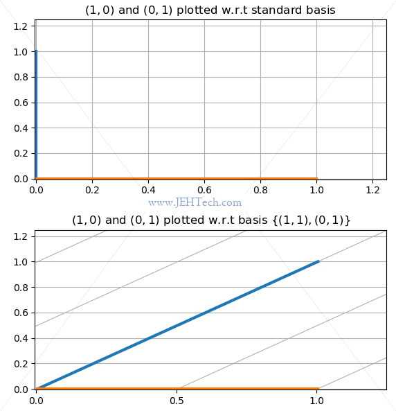
The standard basis in aren't the only basis vectors, as we know. We could use the vectors and , in which case all coordinates are defined as the coefficients of the linear combination of the 2 basis vectors we just chose:
What would our coordinates, , written w.r.t the standard basis be if we wrote them w.r.t our new basis?
With respect to our new basis our x-like and y-like coordinates would be and . So w.r.t our new basis, the coordinates are the coefficients of the basis vectors so we would write . I.e.,
So... the coefficients in the linear combination of the basis vectors for your subspace represent to coordinates w.r.t those chosen basis vectors.
We can see this graphically below, where we see the same two vectors plotted with respect to our different bases. You can see that with the non-standard basis, because everything is expressed as combinations of the non standard basis vectors, our graph's grid has become skewed. This is the effect of the change in basis.
We can generalise the above and introduce some new notation to make things clearer:
If is a subspace of , and if is a basis for , where , then
Where the coordinates of are
Thus in our above examples, we would have said, if was our new basis:
And
When we just write , without the above notation, the standard basis is implied.
Change Of Basis Matrix
We have seen that to construct a transformation matrix we apply the transformation to each column vector of the identity matrix. This means that if is a basis for , then the transformation matrix, , is:
Any vector w.r.t to would be written as:
But here's the interesting thing about the notation. If we were to express as a linear combination of the basis vectors we would write:
Notice how we did not write . The reason for this is that no matter the basis vectors, the linear combination of the coordinates and basis vectors will always result in a vector in , which is expressed by the standard basis.
Thus our change of basis matrix does the following:
Because,
Lets try this using our simple skew example. The change of basis matrix would be:
We know that we transformed to , so is in the standard basis:
Which is exactly what we expected.
In this case, because is square and we know, by definition of its construction, that its column vectors are L.I., that must be invertible. This means we can do the opposite using:
In this case, is trivially found:
So,
Which, is again what we expect. Happy days :)
Invertible Change Of Baisis Matrix
We have seen that if is a basis and its vectors are the column vectors of a matrix , then is the transformation matrix that does the change of basis - it is the change-of-basis matrix:
If is square, then because its columns are L.I. (because they're a basis), we can say that:
And therefore:
Transformation Matrix w.r.t A Basis
Let be , such that . If transforms w.r.t. the standard basis to a vector , then there is a transform that transforms to , where is a basis for .
Lets write this other transform as . We know , so we can write:
Therefore, is the transformation matrix of w.r.t the basis .
Note, at the point, that is some random transform... maybe we're rotating vectors, scaling them or something. is not trying to change basis... it is just a transformation that works on vectors expressed w.r.t. a specific basis.
To change basis, we need a change of basis matrix. We saw in the previous section that , so we know that we can go from any vector w.r.t. the standard basis to the same vector w.r.t. to any other basis, where the basis is the column vectors of .
This means that so far we have:
Thus:
Where is our change of basis matrix and is our transformation matrix w.r.t to basis . is w.r.t. !!
Sal presents this graph which is an excellent summary:
Changing Coordinate Systems To Help Find A Transform Matrix
Sal gives the example of finding the transform for a a reflection in a line, . Normally we would apply the transform to the identity matrix, "I", to get the transformation matrix, :
We could try to figure out using trig but it would be difficult and doesn't scale well into 3D and would be very very difficult in higher dimensions!
But, if we use as our first basis vector and as our second basis vector and express our space with respect to this basis, then the problem becomes taking a reflection in the horizontal axis, which is bar far a simpler problem to solve!
If we wanted to reflect , then we reflect in the horizontal axis. To do this all we have to do is negate the y-value in the vector . Nice!
So,
The transform is thus:
I.e.,
From this we get:
Now we can transform , which is , back to because we know that , so happily we can now calculate the original transform!
Orthonormal Basis
If all vectors in a basis are unit length and are orthogonal to each other, then we call this basis orthonormal. Because all the vectors are orthogonal to eachother, they are also independent.
Orthonormal basis make good coordinate systems, but as Sal asks, "What does good mean?". If is an orthonormal basis for a subspace , and , then we can say, by definition:
We know that can be the only non-zero quantity because by definition all other vectors are perpendicular to , so their dot products with must be zero. Therefore we can say that:
And why is this good?
Well, and may be hard to find, especially if is not invertible. Then we would have to solve for . This method of using , which only holds for orthonormal basis, however, just lets us do:
This is MUCH EASIER! This is why orthonomrla basis are "good": it is easy to figure out coordinates!
Projection Onto Subspace With Orthonormal Basis
We had previously seen that a projection onto any subspace can be defined as:
Where the column vectors of are the basis vectors for the subspace that we are projecting onto. However, when the basis is orthonormal, this reduces to:
Much nicer :) Another reason why orthonormal basis are "good"
Orthogonal Matricies Preserve Angles And Lengths
An orthogonal matrix is one whos columns and rows are orthonomal vectors of the same number of elements, i.e., they're square. This means
that:
This also means that:
This makes finding the inverse of the matrix much, much easier!
Such matricies also preserve angles and lengths when they are used as transformation matricies. Thus, if we tranformed two different vectors, then angle between them would stay the same and their lengths would too. In other words, what we are saying is, that under this transform:
We can see that such a transform preserves lengths:
We can, in a similar manner, see that such a transform preserves angles:
Make Any Basis Orthonormal: The Gram-Schmidt Process
Any basis can be transformed into an orthonormal basis using the Gram-Schidt processes. It is a recursive method.
If is a basis , for , the vectors must be L.I., but not necessarily perpendicular. To make them perpendicular and of unit length, create a subspace :
Next create a subspace, as follows:
We know that we can re-write as the sum of two vectors from a subspace and its perpendicular subspace.
We can write:
We also know
And
Because has been made an orthonormal basis, we know that
So,
We can now, again, normalise to become in the same way as before:
And now we can re-write as the orthonormal basis
We can keep repeating this process for all the vectors in the basis until they are normalised.
Eigen Vectors & Eigen Values
If and , then is an eigen vector and is an eigen value.
We can note from the above definition that only scales the vector . Because vectors are only scaled, the angles between them must also be maintained. This is a little reminiscent of the section on orthogonal matricies preserving angles and lengths, except in this case, lengths are not maintined.
If and a solution exists with , then eigen vectors and values exist.
We know that so is non trivial. We saw in the section on
null spaces that the column vectors of a matrix A are LI if and only if .
This means that the column vectors of must not be L.I. This means that the matrix is not invertible, which means that there must be some for which (see the section on determinants - a matrix is only invertible iff ).
has solutions for non-zero 's iff . By using this we can solve for .
Properties
Eigen vectors can only be found for square matricies.
Not every square matrix has eigen vectors, but if it does and it is an nxn matrix, then there are n eigen vectors.
When you find an eigen vector it is normally a good idea to normalise it.
Example 1
An example...
is an eigen value of .
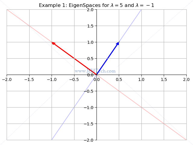
We saw above how . Thus for any eigen value, the eigen vectors, that correspont to it are the null space . This is called the eigen space - denoted .
Thus for :
From here we can say, therefore:
Solve using augmented matrix
Therefore,
And in the same way we can find out that
We can plot these:
Sal presents a second example...
Remember, the e.v. equation is , so in this case we have:
We can use the rule of Sarrus to solve this:
Simplifying this a little we get:
This means that the roots are either or
As before, we know that .
For :
Solve using augmented matrix:
Thus:
From which we can say:
We can do the same for , where we would get the result
We can note that and are perpendicular. However, this need
not be the case in general [Ref].
Showing That Eigen Basis Are Good Coorinate Systems
It can be shown that if a transformation matrix has and least L.I. eignevectors then we can form a basis
where , such that the transfirmation in this new basis representation
can be written as:
Recall in the section on transformation matricies w.r.t a basis Sal Khan's summary graph:
We can show this as follows:
TODO
 The set of all linear combinations of a set of vectors